$\newcommand{\dede}[2]{\frac{\partial #1}{\partial #2} }
\newcommand{\dd}[2]{\frac{d #1}{d #2}}
\newcommand{\divby}[1]{\frac{1}{#1} }
\newcommand{\typing}[3][\Gamma]{#1 \vdash #2 : #3}
\newcommand{\xyz}[0]{(x,y,z)}
\newcommand{\xyzt}[0]{(x,y,z,t)}
\newcommand{\hams}[0]{-\frac{\hbar^2}{2m}(\dede{^2}{x^2} + \dede{^2}{y^2} + \dede{^2}{z^2}) + V\xyz}
\newcommand{\hamt}[0]{-\frac{\hbar^2}{2m}(\dede{^2}{x^2} + \dede{^2}{y^2} + \dede{^2}{z^2}) + V\xyzt}
\newcommand{\ham}[0]{-\frac{\hbar^2}{2m}(\dede{^2}{x^2}) + V(x)}
\newcommand{\konko}[2]{^{#1}\space_{#2}}
\newcommand{\kokon}[2]{_{#1}\space^{#2}} $
# Content
$\newcommand{\L}{\mathcal L}$
$\newcommand{\lrangle}[1]{\langle #1 \rangle}$
$\newcommand{\xton}[1]{x_{1}, \ldots, x_{#1}}$
$\newcommand{\pmatrix}[1]{ \begin{pmatrix} #1 \end{pmatrix}}$
$\newcommand{\ad}{{\hat{a}^{\dagger}}}$
$\newcommand{\a}{\hat{a}}$
# Bose gasses
We want to figure out what happens if we cool down a gas of bosons to near their ground state.
We know that the pauli principle does not apply, so we expect some strange quantum behaviour to occur.
## Pair correlation
##### Pair correlation
Looking at the form of the density operator
$\bra \phi \rho \ket \phi = \bra \phi \Psi^{\dagger}\Psi \ket \phi = \frac{1}{V} \sum\limits_{k_{1},k_{2}} e^{-i(k_{1}-k_{2})x} \bra\phi \ad_{k_{1}} \a_{k_{2}} \ket \phi$
We notice that there is quite a nice place where we could take our intuitions about the mode correlation and plug them in.
Using a bit of math trickery we thus write
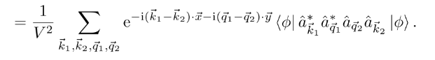
$$\frac{N^{2}}{V^{2}}g(x-y) = \bra \phi \Psi^{\dagger}_{x} \Psi^{\dagger}_{y} \Psi_{y} \Psi_{x} \ket \phi$$
Figuring out what the overlap using the creation operators is and after a buch of maths.
The final result is then:
$$\frac{N^{2}}{V^{2}}g(x-y) = \frac{N^{2}}{V^{2}} + \left| \frac{1}{V} \sum\limits_{k}e^{-ik(x-y)} n_{k} \right|^{2} - \frac{1}{V^{2}} \sum\limits_{k}n_{k}(n_{k}+1)$$
## Boson collective states
### Coherent states
Consider the state where all particles are in the same mode
$$\frac{N^{2}}{V^{2}}g(x-y) = \frac{N^{2}}{V^{2}} + \left|\frac{1}{V} \sum\limits_{k} e^{ik(x-y) } N \delta_{k,k_{0}}\right|^{2} - N\frac{N+1}{V^{2}}$$
$$\frac{N^{2}}{V^{2}}g(x-y) = \frac{N^{2}}{V^{2}} + \frac{N^{2}}{V^{2}} - N\frac{N+1}{V^{2}} = \frac{N(N-1)}{V^{2}}$$
We see that the correlation is constant.
That means that there is no correlation between particles.
This might be slightly un-intuitive. If they are all in the same state, shouldn't they be **fully** correlated?
The thing is that in the case where all particles are in the same state, the maximum confusion we can have is due to the quantum wave function.
This confusion we cannot reduce without breaking uncertainty.
### Gaussian incoherent states
We consider the state:
$n_{k} = \frac{N}{V} \frac{(2\pi)^{3}}{(b\sqrt{\pi})^{3}}e^\frac{-(k-k_{0})^{2}}{b^{2}}$
We will assume large $V$ so we can replace the sum over an integral
$$\frac{N^{2}}{V^{2}}g(x-y) = \frac{N^{2}}{V^{2}} + \left|\int \frac{d^{3}k}{(2\pi)^{3}} e^{ik(x-y) } \frac{N}{V} \frac{(2\pi)^{3}}{(b\sqrt{\pi})^{3}}e^{\frac{-(k-k_{0})^{2}}{b^{2}}} \right|^{2} - \frac{N^{2}}{V^{2}} \mathcal O(\frac{1}{V})$$
Doing the gaussian integral
we get:
$$\frac{N^{2}}{V^{2}}g(x-y) = \frac{N^{2}}{V^{2}}\left[ 1 + e^{\frac{-b^{2}(x-y)^{2}}{2}} + \mathcal O(\frac{1}{V})\right]$$
Which is large for $x$ close to $y$ and small far away:
This means that photons (in this state) tend to bunch up close to eachother.
This effect is called Hanbury-Brown-Twiss and paved the way to quantum optics (working with the quantum correlations in light).
The effect can be used to measure the coherence properties of a light source.
This can then for example be used to find the diameter of a star (beyond the resolution limit)
### What do we learn from this
Depending on the collective state, measurements can become spatially correlated. For example in the gaussian incoherent state. The correlation starts high, but then lowers to a constant level. Even "uncorrelated" states still can have non-zero pair correlation. The point is that this correlation has no spatial dependence.
Meaning that every pair of measurements is just as correlated (/ uncorrelated) as any other pair.
# Bose Einstein Condensation
Now that we have seen some interesting collective states we would like to see what kinds of states can form naturally.
### Non-interacting Bosons
The simplest model is considering non-interacting particles. So the only effects we will see are caused by symmetry and individual particles.
The Hamiltonian will thus have only kinetic energy:
$$\hat H = \sum_{i}^{N} \frac{\vec p_{i}^{2}}{2m} = \sum\limits_{i}^{N} E_{\vec p_{i}}$$
We now consider that the particles are confined to a box with side-length $L$.
We now get quantisation conditions (like for the particle in the square well).
$\vec p = \frac{2\pi\hbar}{L} \vec n$
with $\vec n \in \mathbb{Z}^{3}$
Instead of adding up the individual energy of each particle we can also group them by momentum (that is now quantized).
$E = \sum\limits_{\vec p} n_{\vec p} E_{\vec p}$
This suggests that a good collective state basis is the number state basis. We thus write our collective state as:
$$\ket \psi_{\{n_{\vec p}\}}$$
With $\{ n_{p}\}$ a multiindex (i.e. a list of numbers, which specifies how many particles are in the state with momentum $\vec p$)
# Repetition Theory of Heat
In theory of heat you have seen that boundary conditions on thermodynamical systems can be imposed by choosing the correct ensemble.
One of the most common ensembles is the canonical ensemble, which is used for constant volume temperature and particle number.
In the statistical mechanics picture the ensembles were always specified by a probability of a state and a normalization constant. The normalisation constant $Z(\beta)$ is called the partition function.
$pr[E_{i}] = \frac{1}{Z(\beta)}e^{-\beta E_{i}}$
Finding the partition function is then easy, because all probabilities need to add up to $1$.
$$Z(\beta) = \sum\limits_{i}e^{-\beta E_{i}}$$
In our case we can simply plug in the total system energy. We also replace the index $i$ with the more convenient multiindex.
Additionally we are going to generalize the partition function to any $N$
$$Z_{N}(\beta) = \sum\limits_{\{n_{\vec p}\},N} e^{-\beta\sum\limits_{p}n_{p}E_{p}}$$
(The $N$ in the sum is only notation that helps us remember how big our multiindex is)
### Using the canonical ensemble.
One thing we can do from the canonical partition function is extract expectation values.
#### Mini-repe probability
Let's say we decide to waste our money by going to the casino. To find out how much money we are expected to loose we need to calculate the expected value.
For this we need to multiply the probability of an event with it's outcome.
Consider the following scenario:
$0.1 \to 10CHF$
$0.2 \to -100CHF$
$0.69 \to 1CHF$
$0.01 \to 1000CHF$
$cash_{exp} = 0.1 \cdot 10 + 0.2 \cdot -100 + 0.69 \cdot 1 + 0.01 \cdot 1000 = -8.31 CHF$
More generally we have:
$$cash_{exp}= \sum\limits_{options}p_{o} \cdot cash_{o}$$
#### Concept question
Which equations are correct?
**a)** $\langle \beta \rangle = \frac{1}{Z} \sum\limits \beta e^{-\beta E_{i}}$
**b)** $\langle E \rangle =\frac{1}{Z} \sum\limits E_{i} e^{-\beta E_{i}}$
**c)** $\langle \vec p \rangle = \frac{1}{Z} \sum\limits \vec p_{i} e^{-\beta E_{p_{i}}}$
All are correct.
**a)** Beta does not depend on $i$, can thus be taken out of the sum. The sum normalizes to $Z$
**b)** Correct
**c)** Correct
#### Extracting usefull values:
In statistical physics there is basically one universal trick, which is taking a derivative of a sum.
Let's say we wanted to know the expected energy in a system at temperature $T$.
We realize that taking a derivative of $Z$ with respect to $\beta$ gives the form for the energy expectation:
$\dede{Z}{\beta} = \sum\limits \dede{}{\beta} e^{-\beta E_{i}} = \sum\limits -E_{i} e^{-\beta E_{i}}$
We note that the only thing missing here is the minus sign and the normalisation by $Z$.
$-\frac{1}{Z}\dede{Z}{\beta} = \frac{1}{Z}\sum\limits E_{i} e^{-\beta E_{i}} = \langle E\rangle$
We now use one last trick which is $\dede{}{x} \log(f(x)) = \frac{1}{x}\dede{f(x)}{x}$
And thus get:
$$\langle E \rangle = -\dede{\log(Z)}{\beta}$$
### Changing particle numbers:
We learned in the previous lectures that bosons can be created and destroyed, thus we cannot have a fixed number of particles.
We thus need to use the grand canonical ensemble, which has constant $V,T, \mu$
The chemical potential specifies how much energy it takes/releases to create $N$ particles.
The even more usefull quantity is the fugacity $z = e^{\beta\mu}$, which specifies the probability of finding a new particle.
The total grand partition function is thus: $$\Xi (\beta, \mu) = \sum\limits_{N}^{\infty}\underbrace{z^{N}}_{e^{\beta\mu N}}Z_{N}(\beta)$$
We can again use the stat-phys trick and extract particle numbers, by realizing that taking the derivative Wrt $\beta\mu$
$$\langle N \rangle =\frac{1}{\beta} \dede{}{\mu} \log \Xi$$
For our system additional particles cost exactly $E_{p}$ so the expected number of particles at $p$ are:
$\frac{1}{\beta} \dede{}{(-E_{p})}\log \Xi = \langle n_{p}\rangle$
### Bose einstein statistics
By doing some math (that you'll see in the exercise) we can get to a much nicer form of $\Xi$:
$$\Xi(\beta, \mu) = \prod\limits_{\vec p} \frac{1}{{1-ze^{-\beta E_{\vec p}}}}$$
We like this form, because the log of this will be a sum of logs.
$\log(\Xi) = \sum\limits_{\vec p} \log(\frac{1}{1-ze^{-\beta E_{p}}})$
Thus the expected number of particles in momentum state $p$ is:
$$\langle n_{p}\rangle = -\frac{1}{\beta} \sum\limits_{p}\dede{}{E_{p}}\log \frac{1}{1-ze^{-\beta E_{p}}} = - \frac{1}{\beta}(1-ze^{-\beta E_{p}}) \dede{}{E_{p}}\frac{1}{1-ze^{-\beta E_{p}}}$$
$$ = \frac{1}{\beta}(1-ze^{-\beta E_{p}}) \frac{1}{(1-ze^{-\beta E_{p}})^{2}} ze^{-\beta E_{p}}\cdot \beta$$
$$ = \frac{1}{1-ze^{-\beta E_{p}}} ze^{-\beta E_{p}} = \frac{1}{z^{-1}e^{\beta E_{p}} - 1}$$
Which is the **Bose Einstein Distribution**
Particularly interesting for us is going to be the case $p = 0$
$$\langle n_{0} \rangle = \frac{1}{z^{-1}-1} = \frac{z}{1-z}$$
#### Bonus fermi statistics
### Condensation
We now consider the density of particles:
$$\frac{\langle N\rangle}{V} = \frac{1}{V}\sum\limits_{p} \langle n_{p}\rangle$$
We will now consider $V \to \infty$ so we can replace the sum with the integral
$\frac{1}{V} \sum\limits_{p} \to \frac{1}{(2\pi\hbar)^{3}}\int d^{3} p$
The only problem is the zero component, as in the integral it will have zero measure. So we treat it seperately:
$$\frac{\lrangle{N}}{V} \leq \frac{4\pi}{(2\pi\hbar)^{3}}\int_{0}^{\infty} dp p^{2} \lrangle {n_{p}}+ \frac{1}{V} \frac{z}{1-z}$$
The integral is actually not exact, but it is an upper bound.
We now want to see what we can say about the occupation of the $p=0$ state.
$$\frac{\langle N \rangle }{V} - \int\ldots \leq \frac{1}{V} \frac{z}{1-z} = \frac{\langle n_{0}\rangle}{V}$$
We see that if $\frac{\langle N\rangle}{V}$ is equal to the integral, we do not have significant occupation of the ground state.
However if we increase the density, without changing $z$ or $\beta$ we will reach a point, where $\langle n_{0} \rangle$ will be significantly populated.
The same is true if we keep the density but $T \to 0$. We start to condense into the ground state. This phenomenon is called bose einstein condensation, and can only happen for bosons.
# Quick topic recap
I'll give you a bit of time to do a survey about what topics to cover in the last TA lesson. To help you know what topics we even covered this is a quick speed-run of (almost) everything we covered:
### Repetition
#### Linalg II
- Tensors
- Tensor algebras
- Dual spaces
#### General Mechanics
- Lagrangian & Hamiltonian mechanics
- Picture changes (Heisenber, Schödinger, Interaction)
#### MMP I
- Spherical Harmonics
#### MMP II
- Lie Algebra & Groups
- Campbell Baker Hausdorff
#### Physics II
- Maxwell equations
- Vector potential
- Gague Freedoms
#### QM I
- The harmonic oscillator
- Position/ Momentum basis
-
### Path integrals
- Propagator $U$
- Propagation Kernel
- Explicit spatial propagator
- Path integral
- principle of interfering action
- Classical correspondence to principle of least action
- Commutation & Time ordering
- Classical limit & Path measurements
- Euclidean Path integrals
### Scattering Theory
- Differential cross-section
- Probability fluxes/currents
- Greens functions
- The Lipman Schwinger Equation
- Fraunhofer approximation
- Born approximation
- Partial wave analysis
- Spherical harmonics
### Light Matter Interactions
- Fermis Golden Rule
- Minimal Coupling
- Dipole Approximation
- Selection rules
- Second quantization
- Field quantisation
- Quadratures
- Absorbtion & Emission/ Einstein coefficients
### Identical Particles
- Indistinguishability
- Bosons vs Fermions
- Symmetrization
- Slatter determinand
- Pauli principle
- Triplet vs Singlet
- Wave-function vs spin symmetry
- Scattering of identical particles
- Fock space
- Mode creation/anihilation
- Field creation/anihilation
- Density operator
- Bose gases
- Pair correlation
- Bose Einstein Condensation
- Collective states
### Quantum foundations
- Bell states
- EPR paradox
- CSHS game
- Entanglement & Non-signaling
# Feedback & Repetition
https://nc.zura.ch/apps/forms/s/FPkm5o8YtrCNrkjzMTszyfdy
 Figuring out what the overlap using the creation operators is and after a buch of maths.
The final result is then:
$$\frac{N^{2}}{V^{2}}g(x-y) = \frac{N^{2}}{V^{2}} + \left| \frac{1}{V} \sum\limits_{k}e^{-ik(x-y)} n_{k} \right|^{2} - \frac{1}{V^{2}} \sum\limits_{k}n_{k}(n_{k}+1)$$
## Boson collective states
### Coherent states
Consider the state where all particles are in the same mode
$$\frac{N^{2}}{V^{2}}g(x-y) = \frac{N^{2}}{V^{2}} + \left|\frac{1}{V} \sum\limits_{k} e^{ik(x-y) } N \delta_{k,k_{0}}\right|^{2} - N\frac{N+1}{V^{2}}$$
$$\frac{N^{2}}{V^{2}}g(x-y) = \frac{N^{2}}{V^{2}} + \frac{N^{2}}{V^{2}} - N\frac{N+1}{V^{2}} = \frac{N(N-1)}{V^{2}}$$
We see that the correlation is constant.
That means that there is no correlation between particles.
This might be slightly un-intuitive. If they are all in the same state, shouldn't they be **fully** correlated?
The thing is that in the case where all particles are in the same state, the maximum confusion we can have is due to the quantum wave function.
This confusion we cannot reduce without breaking uncertainty.
### Gaussian incoherent states
We consider the state:
$n_{k} = \frac{N}{V} \frac{(2\pi)^{3}}{(b\sqrt{\pi})^{3}}e^\frac{-(k-k_{0})^{2}}{b^{2}}$
We will assume large $V$ so we can replace the sum over an integral
$$\frac{N^{2}}{V^{2}}g(x-y) = \frac{N^{2}}{V^{2}} + \left|\int \frac{d^{3}k}{(2\pi)^{3}} e^{ik(x-y) } \frac{N}{V} \frac{(2\pi)^{3}}{(b\sqrt{\pi})^{3}}e^{\frac{-(k-k_{0})^{2}}{b^{2}}} \right|^{2} - \frac{N^{2}}{V^{2}} \mathcal O(\frac{1}{V})$$
Doing the gaussian integral
we get:
$$\frac{N^{2}}{V^{2}}g(x-y) = \frac{N^{2}}{V^{2}}\left[ 1 + e^{\frac{-b^{2}(x-y)^{2}}{2}} + \mathcal O(\frac{1}{V})\right]$$
Which is large for $x$ close to $y$ and small far away:
This means that photons (in this state) tend to bunch up close to eachother.
This effect is called Hanbury-Brown-Twiss and paved the way to quantum optics (working with the quantum correlations in light).
The effect can be used to measure the coherence properties of a light source.
This can then for example be used to find the diameter of a star (beyond the resolution limit)
### What do we learn from this
Depending on the collective state, measurements can become spatially correlated. For example in the gaussian incoherent state. The correlation starts high, but then lowers to a constant level. Even "uncorrelated" states still can have non-zero pair correlation. The point is that this correlation has no spatial dependence.
Meaning that every pair of measurements is just as correlated (/ uncorrelated) as any other pair.
# Bose Einstein Condensation
Now that we have seen some interesting collective states we would like to see what kinds of states can form naturally.
### Non-interacting Bosons
The simplest model is considering non-interacting particles. So the only effects we will see are caused by symmetry and individual particles.
The Hamiltonian will thus have only kinetic energy:
$$\hat H = \sum_{i}^{N} \frac{\vec p_{i}^{2}}{2m} = \sum\limits_{i}^{N} E_{\vec p_{i}}$$
We now consider that the particles are confined to a box with side-length $L$.
We now get quantisation conditions (like for the particle in the square well).
$\vec p = \frac{2\pi\hbar}{L} \vec n$
with $\vec n \in \mathbb{Z}^{3}$
Instead of adding up the individual energy of each particle we can also group them by momentum (that is now quantized).
$E = \sum\limits_{\vec p} n_{\vec p} E_{\vec p}$
This suggests that a good collective state basis is the number state basis. We thus write our collective state as:
$$\ket \psi_{\{n_{\vec p}\}}$$
With $\{ n_{p}\}$ a multiindex (i.e. a list of numbers, which specifies how many particles are in the state with momentum $\vec p$)
# Repetition Theory of Heat
In theory of heat you have seen that boundary conditions on thermodynamical systems can be imposed by choosing the correct ensemble.
One of the most common ensembles is the canonical ensemble, which is used for constant volume temperature and particle number.
In the statistical mechanics picture the ensembles were always specified by a probability of a state and a normalization constant. The normalisation constant $Z(\beta)$ is called the partition function.
$pr[E_{i}] = \frac{1}{Z(\beta)}e^{-\beta E_{i}}$
Finding the partition function is then easy, because all probabilities need to add up to $1$.
$$Z(\beta) = \sum\limits_{i}e^{-\beta E_{i}}$$
In our case we can simply plug in the total system energy. We also replace the index $i$ with the more convenient multiindex.
Additionally we are going to generalize the partition function to any $N$
$$Z_{N}(\beta) = \sum\limits_{\{n_{\vec p}\},N} e^{-\beta\sum\limits_{p}n_{p}E_{p}}$$
(The $N$ in the sum is only notation that helps us remember how big our multiindex is)
### Using the canonical ensemble.
One thing we can do from the canonical partition function is extract expectation values.
#### Mini-repe probability
Let's say we decide to waste our money by going to the casino. To find out how much money we are expected to loose we need to calculate the expected value.
For this we need to multiply the probability of an event with it's outcome.
Consider the following scenario:
$0.1 \to 10CHF$
$0.2 \to -100CHF$
$0.69 \to 1CHF$
$0.01 \to 1000CHF$
$cash_{exp} = 0.1 \cdot 10 + 0.2 \cdot -100 + 0.69 \cdot 1 + 0.01 \cdot 1000 = -8.31 CHF$
More generally we have:
$$cash_{exp}= \sum\limits_{options}p_{o} \cdot cash_{o}$$
#### Concept question
Which equations are correct?
**a)** $\langle \beta \rangle = \frac{1}{Z} \sum\limits \beta e^{-\beta E_{i}}$
**b)** $\langle E \rangle =\frac{1}{Z} \sum\limits E_{i} e^{-\beta E_{i}}$
**c)** $\langle \vec p \rangle = \frac{1}{Z} \sum\limits \vec p_{i} e^{-\beta E_{p_{i}}}$
#### Extracting usefull values:
In statistical physics there is basically one universal trick, which is taking a derivative of a sum.
Let's say we wanted to know the expected energy in a system at temperature $T$.
We realize that taking a derivative of $Z$ with respect to $\beta$ gives the form for the energy expectation:
$\dede{Z}{\beta} = \sum\limits \dede{}{\beta} e^{-\beta E_{i}} = \sum\limits -E_{i} e^{-\beta E_{i}}$
We note that the only thing missing here is the minus sign and the normalisation by $Z$.
$-\frac{1}{Z}\dede{Z}{\beta} = \frac{1}{Z}\sum\limits E_{i} e^{-\beta E_{i}} = \langle E\rangle$
We now use one last trick which is $\dede{}{x} \log(f(x)) = \frac{1}{x}\dede{f(x)}{x}$
And thus get:
$$\langle E \rangle = -\dede{\log(Z)}{\beta}$$
### Changing particle numbers:
We learned in the previous lectures that bosons can be created and destroyed, thus we cannot have a fixed number of particles.
We thus need to use the grand canonical ensemble, which has constant $V,T, \mu$
The chemical potential specifies how much energy it takes/releases to create $N$ particles.
The even more usefull quantity is the fugacity $z = e^{\beta\mu}$, which specifies the probability of finding a new particle.
The total grand partition function is thus: $$\Xi (\beta, \mu) = \sum\limits_{N}^{\infty}\underbrace{z^{N}}_{e^{\beta\mu N}}Z_{N}(\beta)$$
We can again use the stat-phys trick and extract particle numbers, by realizing that taking the derivative Wrt $\beta\mu$
$$\langle N \rangle =\frac{1}{\beta} \dede{}{\mu} \log \Xi$$
For our system additional particles cost exactly $E_{p}$ so the expected number of particles at $p$ are:
$\frac{1}{\beta} \dede{}{(-E_{p})}\log \Xi = \langle n_{p}\rangle$
### Bose einstein statistics
By doing some math (that you'll see in the exercise) we can get to a much nicer form of $\Xi$:
$$\Xi(\beta, \mu) = \prod\limits_{\vec p} \frac{1}{{1-ze^{-\beta E_{\vec p}}}}$$
We like this form, because the log of this will be a sum of logs.
$\log(\Xi) = \sum\limits_{\vec p} \log(\frac{1}{1-ze^{-\beta E_{p}}})$
Thus the expected number of particles in momentum state $p$ is:
$$\langle n_{p}\rangle = -\frac{1}{\beta} \sum\limits_{p}\dede{}{E_{p}}\log \frac{1}{1-ze^{-\beta E_{p}}} = - \frac{1}{\beta}(1-ze^{-\beta E_{p}}) \dede{}{E_{p}}\frac{1}{1-ze^{-\beta E_{p}}}$$
$$ = \frac{1}{\beta}(1-ze^{-\beta E_{p}}) \frac{1}{(1-ze^{-\beta E_{p}})^{2}} ze^{-\beta E_{p}}\cdot \beta$$
$$ = \frac{1}{1-ze^{-\beta E_{p}}} ze^{-\beta E_{p}} = \frac{1}{z^{-1}e^{\beta E_{p}} - 1}$$
Which is the **Bose Einstein Distribution**
Particularly interesting for us is going to be the case $p = 0$
$$\langle n_{0} \rangle = \frac{1}{z^{-1}-1} = \frac{z}{1-z}$$
#### Bonus fermi statistics
### Condensation
We now consider the density of particles:
$$\frac{\langle N\rangle}{V} = \frac{1}{V}\sum\limits_{p} \langle n_{p}\rangle$$
We will now consider $V \to \infty$ so we can replace the sum with the integral
$\frac{1}{V} \sum\limits_{p} \to \frac{1}{(2\pi\hbar)^{3}}\int d^{3} p$
The only problem is the zero component, as in the integral it will have zero measure. So we treat it seperately:
$$\frac{\lrangle{N}}{V} \leq \frac{4\pi}{(2\pi\hbar)^{3}}\int_{0}^{\infty} dp p^{2} \lrangle {n_{p}}+ \frac{1}{V} \frac{z}{1-z}$$
The integral is actually not exact, but it is an upper bound.
We now want to see what we can say about the occupation of the $p=0$ state.
$$\frac{\langle N \rangle }{V} - \int\ldots \leq \frac{1}{V} \frac{z}{1-z} = \frac{\langle n_{0}\rangle}{V}$$
We see that if $\frac{\langle N\rangle}{V}$ is equal to the integral, we do not have significant occupation of the ground state.
However if we increase the density, without changing $z$ or $\beta$ we will reach a point, where $\langle n_{0} \rangle$ will be significantly populated.
The same is true if we keep the density but $T \to 0$. We start to condense into the ground state. This phenomenon is called bose einstein condensation, and can only happen for bosons.
# Quick topic recap
I'll give you a bit of time to do a survey about what topics to cover in the last TA lesson. To help you know what topics we even covered this is a quick speed-run of (almost) everything we covered:
### Repetition
#### Linalg II
- Tensors
- Tensor algebras
- Dual spaces
#### General Mechanics
- Lagrangian & Hamiltonian mechanics
- Picture changes (Heisenber, Schödinger, Interaction)
#### MMP I
- Spherical Harmonics
#### MMP II
- Lie Algebra & Groups
- Campbell Baker Hausdorff
#### Physics II
- Maxwell equations
- Vector potential
- Gague Freedoms
#### QM I
- The harmonic oscillator
- Position/ Momentum basis
-
### Path integrals
- Propagator $U$
- Propagation Kernel
- Explicit spatial propagator
- Path integral
- principle of interfering action
- Classical correspondence to principle of least action
- Commutation & Time ordering
- Classical limit & Path measurements
- Euclidean Path integrals
### Scattering Theory
- Differential cross-section
- Probability fluxes/currents
- Greens functions
- The Lipman Schwinger Equation
- Fraunhofer approximation
- Born approximation
- Partial wave analysis
- Spherical harmonics
### Light Matter Interactions
- Fermis Golden Rule
- Minimal Coupling
- Dipole Approximation
- Selection rules
- Second quantization
- Field quantisation
- Quadratures
- Absorbtion & Emission/ Einstein coefficients
### Identical Particles
- Indistinguishability
- Bosons vs Fermions
- Symmetrization
- Slatter determinand
- Pauli principle
- Triplet vs Singlet
- Wave-function vs spin symmetry
- Scattering of identical particles
- Fock space
- Mode creation/anihilation
- Field creation/anihilation
- Density operator
- Bose gases
- Pair correlation
- Bose Einstein Condensation
- Collective states
### Quantum foundations
- Bell states
- EPR paradox
- CSHS game
- Entanglement & Non-signaling
# Feedback & Repetition
https://nc.zura.ch/apps/forms/s/FPkm5o8YtrCNrkjzMTszyfdy
Figuring out what the overlap using the creation operators is and after a buch of maths.
The final result is then:
$$\frac{N^{2}}{V^{2}}g(x-y) = \frac{N^{2}}{V^{2}} + \left| \frac{1}{V} \sum\limits_{k}e^{-ik(x-y)} n_{k} \right|^{2} - \frac{1}{V^{2}} \sum\limits_{k}n_{k}(n_{k}+1)$$
## Boson collective states
### Coherent states
Consider the state where all particles are in the same mode
$$\frac{N^{2}}{V^{2}}g(x-y) = \frac{N^{2}}{V^{2}} + \left|\frac{1}{V} \sum\limits_{k} e^{ik(x-y) } N \delta_{k,k_{0}}\right|^{2} - N\frac{N+1}{V^{2}}$$
$$\frac{N^{2}}{V^{2}}g(x-y) = \frac{N^{2}}{V^{2}} + \frac{N^{2}}{V^{2}} - N\frac{N+1}{V^{2}} = \frac{N(N-1)}{V^{2}}$$
We see that the correlation is constant.
That means that there is no correlation between particles.
This might be slightly un-intuitive. If they are all in the same state, shouldn't they be **fully** correlated?
The thing is that in the case where all particles are in the same state, the maximum confusion we can have is due to the quantum wave function.
This confusion we cannot reduce without breaking uncertainty.
### Gaussian incoherent states
We consider the state:
$n_{k} = \frac{N}{V} \frac{(2\pi)^{3}}{(b\sqrt{\pi})^{3}}e^\frac{-(k-k_{0})^{2}}{b^{2}}$
We will assume large $V$ so we can replace the sum over an integral
$$\frac{N^{2}}{V^{2}}g(x-y) = \frac{N^{2}}{V^{2}} + \left|\int \frac{d^{3}k}{(2\pi)^{3}} e^{ik(x-y) } \frac{N}{V} \frac{(2\pi)^{3}}{(b\sqrt{\pi})^{3}}e^{\frac{-(k-k_{0})^{2}}{b^{2}}} \right|^{2} - \frac{N^{2}}{V^{2}} \mathcal O(\frac{1}{V})$$
Doing the gaussian integral
we get:
$$\frac{N^{2}}{V^{2}}g(x-y) = \frac{N^{2}}{V^{2}}\left[ 1 + e^{\frac{-b^{2}(x-y)^{2}}{2}} + \mathcal O(\frac{1}{V})\right]$$
Which is large for $x$ close to $y$ and small far away:
This means that photons (in this state) tend to bunch up close to eachother.
This effect is called Hanbury-Brown-Twiss and paved the way to quantum optics (working with the quantum correlations in light).
The effect can be used to measure the coherence properties of a light source.
This can then for example be used to find the diameter of a star (beyond the resolution limit)
### What do we learn from this
Depending on the collective state, measurements can become spatially correlated. For example in the gaussian incoherent state. The correlation starts high, but then lowers to a constant level. Even "uncorrelated" states still can have non-zero pair correlation. The point is that this correlation has no spatial dependence.
Meaning that every pair of measurements is just as correlated (/ uncorrelated) as any other pair.
# Bose Einstein Condensation
Now that we have seen some interesting collective states we would like to see what kinds of states can form naturally.
### Non-interacting Bosons
The simplest model is considering non-interacting particles. So the only effects we will see are caused by symmetry and individual particles.
The Hamiltonian will thus have only kinetic energy:
$$\hat H = \sum_{i}^{N} \frac{\vec p_{i}^{2}}{2m} = \sum\limits_{i}^{N} E_{\vec p_{i}}$$
We now consider that the particles are confined to a box with side-length $L$.
We now get quantisation conditions (like for the particle in the square well).
$\vec p = \frac{2\pi\hbar}{L} \vec n$
with $\vec n \in \mathbb{Z}^{3}$
Instead of adding up the individual energy of each particle we can also group them by momentum (that is now quantized).
$E = \sum\limits_{\vec p} n_{\vec p} E_{\vec p}$
This suggests that a good collective state basis is the number state basis. We thus write our collective state as:
$$\ket \psi_{\{n_{\vec p}\}}$$
With $\{ n_{p}\}$ a multiindex (i.e. a list of numbers, which specifies how many particles are in the state with momentum $\vec p$)
# Repetition Theory of Heat
In theory of heat you have seen that boundary conditions on thermodynamical systems can be imposed by choosing the correct ensemble.
One of the most common ensembles is the canonical ensemble, which is used for constant volume temperature and particle number.
In the statistical mechanics picture the ensembles were always specified by a probability of a state and a normalization constant. The normalisation constant $Z(\beta)$ is called the partition function.
$pr[E_{i}] = \frac{1}{Z(\beta)}e^{-\beta E_{i}}$
Finding the partition function is then easy, because all probabilities need to add up to $1$.
$$Z(\beta) = \sum\limits_{i}e^{-\beta E_{i}}$$
In our case we can simply plug in the total system energy. We also replace the index $i$ with the more convenient multiindex.
Additionally we are going to generalize the partition function to any $N$
$$Z_{N}(\beta) = \sum\limits_{\{n_{\vec p}\},N} e^{-\beta\sum\limits_{p}n_{p}E_{p}}$$
(The $N$ in the sum is only notation that helps us remember how big our multiindex is)
### Using the canonical ensemble.
One thing we can do from the canonical partition function is extract expectation values.
#### Mini-repe probability
Let's say we decide to waste our money by going to the casino. To find out how much money we are expected to loose we need to calculate the expected value.
For this we need to multiply the probability of an event with it's outcome.
Consider the following scenario:
$0.1 \to 10CHF$
$0.2 \to -100CHF$
$0.69 \to 1CHF$
$0.01 \to 1000CHF$
$cash_{exp} = 0.1 \cdot 10 + 0.2 \cdot -100 + 0.69 \cdot 1 + 0.01 \cdot 1000 = -8.31 CHF$
More generally we have:
$$cash_{exp}= \sum\limits_{options}p_{o} \cdot cash_{o}$$
#### Concept question
Which equations are correct?
**a)** $\langle \beta \rangle = \frac{1}{Z} \sum\limits \beta e^{-\beta E_{i}}$
**b)** $\langle E \rangle =\frac{1}{Z} \sum\limits E_{i} e^{-\beta E_{i}}$
**c)** $\langle \vec p \rangle = \frac{1}{Z} \sum\limits \vec p_{i} e^{-\beta E_{p_{i}}}$
#### Extracting usefull values:
In statistical physics there is basically one universal trick, which is taking a derivative of a sum.
Let's say we wanted to know the expected energy in a system at temperature $T$.
We realize that taking a derivative of $Z$ with respect to $\beta$ gives the form for the energy expectation:
$\dede{Z}{\beta} = \sum\limits \dede{}{\beta} e^{-\beta E_{i}} = \sum\limits -E_{i} e^{-\beta E_{i}}$
We note that the only thing missing here is the minus sign and the normalisation by $Z$.
$-\frac{1}{Z}\dede{Z}{\beta} = \frac{1}{Z}\sum\limits E_{i} e^{-\beta E_{i}} = \langle E\rangle$
We now use one last trick which is $\dede{}{x} \log(f(x)) = \frac{1}{x}\dede{f(x)}{x}$
And thus get:
$$\langle E \rangle = -\dede{\log(Z)}{\beta}$$
### Changing particle numbers:
We learned in the previous lectures that bosons can be created and destroyed, thus we cannot have a fixed number of particles.
We thus need to use the grand canonical ensemble, which has constant $V,T, \mu$
The chemical potential specifies how much energy it takes/releases to create $N$ particles.
The even more usefull quantity is the fugacity $z = e^{\beta\mu}$, which specifies the probability of finding a new particle.
The total grand partition function is thus: $$\Xi (\beta, \mu) = \sum\limits_{N}^{\infty}\underbrace{z^{N}}_{e^{\beta\mu N}}Z_{N}(\beta)$$
We can again use the stat-phys trick and extract particle numbers, by realizing that taking the derivative Wrt $\beta\mu$
$$\langle N \rangle =\frac{1}{\beta} \dede{}{\mu} \log \Xi$$
For our system additional particles cost exactly $E_{p}$ so the expected number of particles at $p$ are:
$\frac{1}{\beta} \dede{}{(-E_{p})}\log \Xi = \langle n_{p}\rangle$
### Bose einstein statistics
By doing some math (that you'll see in the exercise) we can get to a much nicer form of $\Xi$:
$$\Xi(\beta, \mu) = \prod\limits_{\vec p} \frac{1}{{1-ze^{-\beta E_{\vec p}}}}$$
We like this form, because the log of this will be a sum of logs.
$\log(\Xi) = \sum\limits_{\vec p} \log(\frac{1}{1-ze^{-\beta E_{p}}})$
Thus the expected number of particles in momentum state $p$ is:
$$\langle n_{p}\rangle = -\frac{1}{\beta} \sum\limits_{p}\dede{}{E_{p}}\log \frac{1}{1-ze^{-\beta E_{p}}} = - \frac{1}{\beta}(1-ze^{-\beta E_{p}}) \dede{}{E_{p}}\frac{1}{1-ze^{-\beta E_{p}}}$$
$$ = \frac{1}{\beta}(1-ze^{-\beta E_{p}}) \frac{1}{(1-ze^{-\beta E_{p}})^{2}} ze^{-\beta E_{p}}\cdot \beta$$
$$ = \frac{1}{1-ze^{-\beta E_{p}}} ze^{-\beta E_{p}} = \frac{1}{z^{-1}e^{\beta E_{p}} - 1}$$
Which is the **Bose Einstein Distribution**
Particularly interesting for us is going to be the case $p = 0$
$$\langle n_{0} \rangle = \frac{1}{z^{-1}-1} = \frac{z}{1-z}$$
#### Bonus fermi statistics
### Condensation
We now consider the density of particles:
$$\frac{\langle N\rangle}{V} = \frac{1}{V}\sum\limits_{p} \langle n_{p}\rangle$$
We will now consider $V \to \infty$ so we can replace the sum with the integral
$\frac{1}{V} \sum\limits_{p} \to \frac{1}{(2\pi\hbar)^{3}}\int d^{3} p$
The only problem is the zero component, as in the integral it will have zero measure. So we treat it seperately:
$$\frac{\lrangle{N}}{V} \leq \frac{4\pi}{(2\pi\hbar)^{3}}\int_{0}^{\infty} dp p^{2} \lrangle {n_{p}}+ \frac{1}{V} \frac{z}{1-z}$$
The integral is actually not exact, but it is an upper bound.
We now want to see what we can say about the occupation of the $p=0$ state.
$$\frac{\langle N \rangle }{V} - \int\ldots \leq \frac{1}{V} \frac{z}{1-z} = \frac{\langle n_{0}\rangle}{V}$$
We see that if $\frac{\langle N\rangle}{V}$ is equal to the integral, we do not have significant occupation of the ground state.
However if we increase the density, without changing $z$ or $\beta$ we will reach a point, where $\langle n_{0} \rangle$ will be significantly populated.
The same is true if we keep the density but $T \to 0$. We start to condense into the ground state. This phenomenon is called bose einstein condensation, and can only happen for bosons.
# Quick topic recap
I'll give you a bit of time to do a survey about what topics to cover in the last TA lesson. To help you know what topics we even covered this is a quick speed-run of (almost) everything we covered:
### Repetition
#### Linalg II
- Tensors
- Tensor algebras
- Dual spaces
#### General Mechanics
- Lagrangian & Hamiltonian mechanics
- Picture changes (Heisenber, Schödinger, Interaction)
#### MMP I
- Spherical Harmonics
#### MMP II
- Lie Algebra & Groups
- Campbell Baker Hausdorff
#### Physics II
- Maxwell equations
- Vector potential
- Gague Freedoms
#### QM I
- The harmonic oscillator
- Position/ Momentum basis
-
### Path integrals
- Propagator $U$
- Propagation Kernel
- Explicit spatial propagator
- Path integral
- principle of interfering action
- Classical correspondence to principle of least action
- Commutation & Time ordering
- Classical limit & Path measurements
- Euclidean Path integrals
### Scattering Theory
- Differential cross-section
- Probability fluxes/currents
- Greens functions
- The Lipman Schwinger Equation
- Fraunhofer approximation
- Born approximation
- Partial wave analysis
- Spherical harmonics
### Light Matter Interactions
- Fermis Golden Rule
- Minimal Coupling
- Dipole Approximation
- Selection rules
- Second quantization
- Field quantisation
- Quadratures
- Absorbtion & Emission/ Einstein coefficients
### Identical Particles
- Indistinguishability
- Bosons vs Fermions
- Symmetrization
- Slatter determinand
- Pauli principle
- Triplet vs Singlet
- Wave-function vs spin symmetry
- Scattering of identical particles
- Fock space
- Mode creation/anihilation
- Field creation/anihilation
- Density operator
- Bose gases
- Pair correlation
- Bose Einstein Condensation
- Collective states
### Quantum foundations
- Bell states
- EPR paradox
- CSHS game
- Entanglement & Non-signaling
# Feedback & Repetition
https://nc.zura.ch/apps/forms/s/FPkm5o8YtrCNrkjzMTszyfdy