$\newcommand{\dede}[2]{\frac{\partial #1}{\partial #2} }
\newcommand{\dd}[2]{\frac{d #1}{d #2}}
\newcommand{\divby}[1]{\frac{1}{#1} }
\newcommand{\typing}[3][\Gamma]{#1 \vdash #2 : #3}
\newcommand{\xyz}[0]{(x,y,z)}
\newcommand{\xyzt}[0]{(x,y,z,t)}
\newcommand{\hams}[0]{-\frac{\hbar^2}{2m}(\dede{^2}{x^2} + \dede{^2}{y^2} + \dede{^2}{z^2}) + V\xyz}
\newcommand{\hamt}[0]{-\frac{\hbar^2}{2m}(\dede{^2}{x^2} + \dede{^2}{y^2} + \dede{^2}{z^2}) + V\xyzt}
\newcommand{\ham}[0]{-\frac{\hbar^2}{2m}(\dede{^2}{x^2}) + V(x)}
\newcommand{\konko}[2]{^{#1}\space_{#2}}
\newcommand{\kokon}[2]{_{#1}\space^{#2}} $
# Content
$\newcommand{\L}{\mathcal L}$
$\newcommand{\lrangle}[1]{\langle #1 \rangle}$
$\newcommand{\xton}[1]{x_{1}, \ldots, x_{#1}}$
$\newcommand{\pmatrix}[1]{ \begin{pmatrix} #1 \end{pmatrix}}$
# Hilbert hotel?
Why is the fock space structure of a bosonic field so complicated?
Why do we nee the tensor algebra $\mathcal F_{S } = \bigoplus_{N=0}^{\infty} S(\mathcal H ^{\otimes N})$.
We can think of quantum mechanical states as being a way to tally superpositions of alternatives.
What I mean by this is that we need two properties:
- Every alternative classical state needs to be encodable
- Adding two alternatives, does not lead to both things happening, but rather a superposition of the two
We previously saw that to represent any $N$-particle state we need $\mathcal H^{\otimes N}$.
Now we can think about how we represent classical alternatives of having $N$ or $M$ quantum particles.
That is we consider the number of particles as a classical value, but the particles themselves can have quantum states.
In this case to represent our options we need an object that holds:
- The number of particles
- Their quantum state
We could for example write the two options as:
- $\Psi_{N} = \ket{N}\ket{x_{1},\ldots ,x_{N}}$
- $\Psi_{M}=\ket{M}\ket{x_{1},\ldots ,x_{M}}$
Note that for now we could actually remove the first part, and still get all the necessary information (because the size of the state vector gives us the information we want)
### Now what?
How do I add those two alternatives?
One way is to take the largest space, and just pad the smaller state with zeros:
- $\ket{N}\ket{x_{1},\ldots ,x_{N}, \underbrace{0 ,\ldots, 0}_{N-M}}$
This would however lead to quite some problems. Because what we are saying with this is that the physics of $N$ particles at $x_{1} \to x_{N}$ is the same as if I added $N-M$ particles, all localized at $0$.
Additionally adding the two states, would lead to strange interferences of the $N$ particles with the first $N$ particles of $\Psi_{M}$
What we actually want is for those spaces to be orthogonal.
One way to write this we actually already did. By saying that $\ket N$ and $\ket M$ label which orthogonal subspace I need to be in, we can have superpositions.
Our states would then look like:
$\Psi_{M}+\Psi_{N} = \ket{N}\ket{x_{1},\ldots ,x_{N}} + \ket{M}\ket{x_{1},\ldots ,x_{M}}$
With the implicit rule, that states with different $\ket M$ cannot be added.
This is often how physicists treat fock spaces (often even removing the $\ket N$ and $\ket M$ because the number of $x$ indices is already enough)
### Making the mathematicians happy
But the actually good way to do it (mathematically) is to force the hilbert space structure (or "the matrix") to not allow strange operations.
For this we simply put states with different $N$, $M$ in orthogonal spaces.
The most efficient way to do this is to simply append the new spaces as new entries to the vector:
$$\Psi_{N} = \left ( \begin{array}{c|c c | c | c } 0 & & & \\ \hline & 0 & 0 & & \\ &0 & 0 \\ \hline & & & \Psi_{N} \\\hline & & & & \Psi_M \\\end{array} \right)$$
This allows us to write superpositions of alternatives with differing $N$.
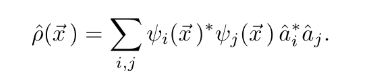
# Density operator
This is now the first time Renner introduces the density operator, we have already previously touched upon it in the exercise class.
The density operator is a generalization of the number operator.
$\rho_{x} = \Psi_{x}^{\dagger}\Psi_{x}$ vs $\hat N = \ad \a$
The general idea is to find the probability to find a particle in some state. To do this we try to destroy the particle and then recreate it. If there was no particle to destroy, we will get zero, and thus cannot recreate the particle
(note that $\ket 0 \neq 0$ )
This $\rho$ is called the density operator, because it's expectation value gives you the probability density of finding a particle at $x$.
### Math
To show this is true (beyond our intuition) we can use the standard qm-basis playbook.
Let's consider two $N$ particle states $\phi,\psi$
$\bra \psi \rho_{x}\ket \phi = \bra\psi \Psi_{x}^{\dagger}\Psi_{x} \ket \psi$
We realize that we would like to insert $x$ eigenstates so we can resolve the field operators.
We consider in the resolution of identity for $N$ particles:
$id_{N} =\int dx_{1} dx_{N} \ket{x_{1} \ldots x_{N}} \bra{x_{1} \ldots x_{N}}$
Now because we know that $\Psi_{x}$ takes $N \to N-1$ particle states, we can simply consider $id_{N-1}$
(note the small abuse of notation. We are not writing the full fock space, rather it is understood that all other alternatives with more or less particles are implied)
$$\bra \psi \rho_{x}\ket \phi = \bra\psi \Psi_{x}^{\dagger}\Psi_{x} \ket \psi = \bra\psi \Psi_{x}^{\dagger}\int dx_{1}dx_{N-1} \ket{\xton{N-1} x} \bra{\xton{N-1}} \Psi_{x} \ket \psi$$
We can pull out the integral (linearity)
$$ = \int dx_{1}dx_{N-1}\bra\psi \Psi_{x}^{\dagger} \ket{\xton{N-1}} \bra{\xton{N-1}} \Psi_{x} \ket \psi$$
We know that $\Psi_{x}^\dagger$ creates a particle at $x$
$$ = N\int dx_{1}dx_{N-1}\bra\psi \ket{\xton{N-1}, x} \bra{\xton{N-1}, x} \ket \psi$$
Now we need to consider all the ways that the states can overlap with the new $x$. We do this by counting the number of times we can have potential overlap. This happens every time, when one of the $x_{i}$ integration variables crosses $x$.
$$ = \sum\limits_{i}^{N}\int dx_{1}dx_{N-1}\bra\psi \ket{\xton{N}} \bra{\xton{N}} \ket \psi \delta(x_{i} - x)$$
We now do something slightly technical. We extend our dirac delta to a distribution acting on operators.
Assuming we already extended it we would like to have
$\delta(\hat x_{i}- x)\ket{\xton{N}} = \delta(x_{i}-x) \ket{\xton{N}}$
I.e. we want it to be compatible with the normal dirac delta.
This will allow us to pull the delta into the integral
$$ = \sum\limits_{i}^{N}\int dx_{1}dx_{N-1}\bra\psi\delta(\hat x_{i} - x) \ket{\xton{N}} \bra{\xton{N}} \ket \psi $$
Why did we do this. Because now $\hat x_{i}$ is no longer an integration variable (it's a distribution).
We can thus take it out of the integral entirely
$$ =\bra\psi \sum\limits_{i}^{N}\delta(\hat x_{i}- x) \underbrace{\int dx_{1}dx_{N-1} \ket{\xton{N}} \bra{\xton{N}}}_{id} \ket \psi $$
We notice the resolution of identity
$$=\bra \psi \sum\limits_{i}^{N} \delta(\hat x_{i}- x) \ket \phi$$
In this form we see directly that we extract for every particle the probability of $\phi$ to be at $x$. And then overlap that with $\psi$
One noteworthy thing is that for $\phi, \psi$ having different numbers of particles, $\delta$ will only stay within the $\phi_N$ block of the matrix.
The overlap will thus always be zero
### Interpretation
If $\phi = \psi$
We see that we count (for every particle) the probability of one of the particles to be at $x$.
That means we calculate the total probability for any particle to be at $x$.
That is exactly the expected density.
# Bose gasses
We want to figure out what happens if we cool down a gas of bosons to near their ground state.
We know that the pauli principle does not apply, so we expect some strange quantum behaviour to occur.
## Pair correlation
To quantify this we introduce the pair correlation function. This function will tell us how "synced up" our particles are.
We first step back and think about what our density operator told us.
$\rho_{x}$ tells us how likely it is for a particle to be at $x$.
Or if we want to be complicated about this. How likely is it that the particle is at $x$ at the same time that it is at $x$. (wooooow)
But there is no reason, why we should not be able to do the same with two particles. For two particles we obviously have two variables $x$ and $y$
The question would now be how likely is it to find one particle at $x$ while the other particle is at $y$.
We first consider an easier model
### Concept question
What is the interpretation of the following operators:
**a)** $\ad \a$
**b)** $\ad_{j}\ad_{i}\a_{i}\a_{j}$
**c)** $\ad_{i}\a_{i}\ad_{j}\a_{j}$
**a)** Number of excitations
**b)** Number of excitations in $i$ times excitations in $j$
**c)** Same as b
In my opinion the nicest interpretation for b happens when we consider only one particle per mode (for example if the two modes are fermionic).
In this case b) checks the probability to find a particle in mode $j$, while there is also a particle in mode $i$.
It correlates the probabilities of $i$ and $j$
### Concept question
What would be the natural way to build the pair correlation function for the field operators?
We know that $\rho_{x} = \Psi^{\dagger}_{x}\Psi_{x}$.
A natural way to expand this would be
$C \cdot g(x,y) = \Psi^{\dagger}_{x}\Psi^{\dagger}_{y}\Psi_{y}\Psi_{x}$.
Because we require symmetry we can even write it as
$C \cdot g(x-y) = \Psi^{\dagger}_{x}\Psi^{\dagger}_{y}\Psi_{y}\Psi_{x}$.
It turns out that this is exactly the right notion.
Because we would like this to be a pair density (and probabilities are unitless)
we set $C = \frac{N^{2}}{V^{2}}$
### Fourier modes
There is a nice way to put the mode picture and the field operator picture together. You have done this in the lecture and I'll only quickly outline the process.
- Take some volume $V$
- Find all modes that fit into $V$
- Do the inverse process that we did when deriving the field operator (fourier transform)
- You now know what the density of a mode is
- Link the addition of particles in real space, to the excitation of modes in fourier space
- The creation and destruction of fourier modes are the $\ad_{i}$ and $\a_{i}$
##### Just density
We first write:
$\phi_{j} = \frac{1}{\sqrt{V}}e^{ik_{j}x}$
We can then write the full state using the multi mode creation operators:
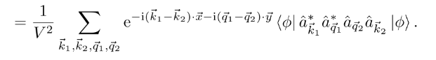
Computing the expectation of a density operator:
$\bra \phi \rho \ket \phi = \bra \phi \Psi^{\dagger}\Psi \ket \phi = \frac{1}{V} \sum\limits_{k_{1},k_{2}} e^{-i(k_{1}-k_{2})x} \bra\phi \ad_{k_{1}} \a_{k_{2}} \ket \phi$
Here we have used the definition of the density operator with respect to the density functions.
Using
$\bra\phi \ad_{k_{1}} \a_{k_{2}} \ket \phi = \delta_{k_{1},k_{2}} n_{k_{1}}$
We can finally write
$\bra \phi \rho \ket \phi = \frac{1}{V}\sum\limits_{k}n_{k} = \frac{N}{V}$
##### Pair correlation
Looking at the form of the density operator
$\bra \phi \rho \ket \phi = \bra \phi \Psi^{\dagger}\Psi \ket \phi = \frac{1}{V} \sum\limits_{k_{1},k_{2}} e^{-i(k_{1}-k_{2})x} \bra\phi \ad_{k_{1}} \a_{k_{2}} \ket \phi$
We notice that there is quite a nice place where we could take our intuitions about the mode correlation and plug them in.
Using a bit of math trickery we thus write
$$\frac{N^{2}}{V^{2}}g(x-y) = \bra \phi \Psi^{\dagger}_{x} \Psi^{\dagger}_{y} \Psi_{y} \Psi_{x} \ket \phi$$
Figuring out what the overlap using the creation operators is and after a buch of maths.
The final result is then:
$$\frac{N^{2}}{V^{2}}g(x-y) = \frac{N^{2}}{V^{2}} + \left| \frac{1}{V} \sum\limits_{k}e^{-ik(x-y)} n_{k} \right|^{2} - \frac{1}{V^{2}} \sum\limits_{k}n_{k}(n_{k}+1)$$
## Boson collective states
### Coherent states
Consider the state where all particles are in the same mode
$$\frac{N^{2}}{V^{2}}g(x-y) = \frac{N^{2}}{V^{2}} + \left|\frac{1}{V} \sum\limits_{k} e^{ik(x-y) } N \delta_{k,k_{0}}\right|^{2} - N\frac{N+1}{V^{2}}$$
$$\frac{N^{2}}{V^{2}}g(x-y) = \frac{N^{2}}{V^{2}} + \frac{N^{2}}{V^{2}} - N\frac{N+1}{V^{2}} = \frac{N(N-1)}{V^{2}}$$
We see that the correlation is constant.
That means that there is no correlation between particles.
This might be slightly unintuitive. If they are all in the same state, shouldn't they be **fully** correlated?
The thing is that in the case where all particles are in the same state, the maximum confusion we can have is due to the quantum wave function.
This confusion we cannot reduce without breaking uncertainty.
### Gaussian incoherent states
We consider the state:
$n_{k} = \frac{N}{V} \frac{(2\pi)^{3}}{(b\sqrt{\pi})^{3}}e^\frac{-(k-k_{0})^{2}}{b^{2}}$
We will assume large $V$ so we can replace the sum over an integral
$$\frac{N^{2}}{V^{2}}g(x-y) = \frac{N^{2}}{V^{2}} + \left|\int \frac{d^{3}k}{(2\pi)^{3}} e^{ik(x-y) } \frac{N}{V} \frac{(2\pi)^{3}}{(b\sqrt{\pi})^{3}}e^{\frac{-(k-k_{0})^{2}}{b^{2}}} \right|^{2} - \frac{N^{2}}{V^{2}} \mathcal O(\frac{1}{V})$$
Doing the gaussian integral
we get:
Which is large for $x$ close to $y$ and small far away:
This means that photons (in this state) tend to bunch up close to eachother.
This effect is called Hanbury-Brown-Twiss and paved the way to quantum optics (working with the quantum correlations in light).
The effect can be used to measure the coherence properties of a light source.
This can then for example be used to find the diameter of a star (beyond the resolution limit)
 This $\rho$ is called the density operator, because it's expectation value gives you the probability density of finding a particle at $x$.
### Math
To show this is true (beyond our intuition) we can use the standard qm-basis playbook.
Let's consider two $N$ particle states $\phi,\psi$
$\bra \psi \rho_{x}\ket \phi = \bra\psi \Psi_{x}^{\dagger}\Psi_{x} \ket \psi$
We realize that we would like to insert $x$ eigenstates so we can resolve the field operators.
We consider in the resolution of identity for $N$ particles:
$id_{N} =\int dx_{1} dx_{N} \ket{x_{1} \ldots x_{N}} \bra{x_{1} \ldots x_{N}}$
This $\rho$ is called the density operator, because it's expectation value gives you the probability density of finding a particle at $x$.
### Math
To show this is true (beyond our intuition) we can use the standard qm-basis playbook.
Let's consider two $N$ particle states $\phi,\psi$
$\bra \psi \rho_{x}\ket \phi = \bra\psi \Psi_{x}^{\dagger}\Psi_{x} \ket \psi$
We realize that we would like to insert $x$ eigenstates so we can resolve the field operators.
We consider in the resolution of identity for $N$ particles:
$id_{N} =\int dx_{1} dx_{N} \ket{x_{1} \ldots x_{N}} \bra{x_{1} \ldots x_{N}}$
 Now because we know that $\Psi_{x}$ takes $N \to N-1$ particle states, we can simply consider $id_{N-1}$
(note the small abuse of notation. We are not writing the full fock space, rather it is understood that all other alternatives with more or less particles are implied)
$$\bra \psi \rho_{x}\ket \phi = \bra\psi \Psi_{x}^{\dagger}\Psi_{x} \ket \psi = \bra\psi \Psi_{x}^{\dagger}\int dx_{1}dx_{N-1} \ket{\xton{N-1} x} \bra{\xton{N-1}} \Psi_{x} \ket \psi$$
We can pull out the integral (linearity)
$$ = \int dx_{1}dx_{N-1}\bra\psi \Psi_{x}^{\dagger} \ket{\xton{N-1}} \bra{\xton{N-1}} \Psi_{x} \ket \psi$$
We know that $\Psi_{x}^\dagger$ creates a particle at $x$
$$ = N\int dx_{1}dx_{N-1}\bra\psi \ket{\xton{N-1}, x} \bra{\xton{N-1}, x} \ket \psi$$
Now we need to consider all the ways that the states can overlap with the new $x$. We do this by counting the number of times we can have potential overlap. This happens every time, when one of the $x_{i}$ integration variables crosses $x$.
$$ = \sum\limits_{i}^{N}\int dx_{1}dx_{N-1}\bra\psi \ket{\xton{N}} \bra{\xton{N}} \ket \psi \delta(x_{i} - x)$$
We now do something slightly technical. We extend our dirac delta to a distribution acting on operators.
Assuming we already extended it we would like to have
$\delta(\hat x_{i}- x)\ket{\xton{N}} = \delta(x_{i}-x) \ket{\xton{N}}$
I.e. we want it to be compatible with the normal dirac delta.
This will allow us to pull the delta into the integral
$$ = \sum\limits_{i}^{N}\int dx_{1}dx_{N-1}\bra\psi\delta(\hat x_{i} - x) \ket{\xton{N}} \bra{\xton{N}} \ket \psi $$
Why did we do this. Because now $\hat x_{i}$ is no longer an integration variable (it's a distribution).
We can thus take it out of the integral entirely
$$ =\bra\psi \sum\limits_{i}^{N}\delta(\hat x_{i}- x) \underbrace{\int dx_{1}dx_{N-1} \ket{\xton{N}} \bra{\xton{N}}}_{id} \ket \psi $$
We notice the resolution of identity
$$=\bra \psi \sum\limits_{i}^{N} \delta(\hat x_{i}- x) \ket \phi$$
In this form we see directly that we extract for every particle the probability of $\phi$ to be at $x$. And then overlap that with $\psi$
One noteworthy thing is that for $\phi, \psi$ having different numbers of particles, $\delta$ will only stay within the $\phi_N$ block of the matrix.
The overlap will thus always be zero
### Interpretation
If $\phi = \psi$
We see that we count (for every particle) the probability of one of the particles to be at $x$.
That means we calculate the total probability for any particle to be at $x$.
That is exactly the expected density.
# Bose gasses
We want to figure out what happens if we cool down a gas of bosons to near their ground state.
We know that the pauli principle does not apply, so we expect some strange quantum behaviour to occur.
## Pair correlation
To quantify this we introduce the pair correlation function. This function will tell us how "synced up" our particles are.
We first step back and think about what our density operator told us.
$\rho_{x}$ tells us how likely it is for a particle to be at $x$.
Or if we want to be complicated about this. How likely is it that the particle is at $x$ at the same time that it is at $x$. (wooooow)
But there is no reason, why we should not be able to do the same with two particles. For two particles we obviously have two variables $x$ and $y$
The question would now be how likely is it to find one particle at $x$ while the other particle is at $y$.
We first consider an easier model
### Concept question
What is the interpretation of the following operators:
**a)** $\ad \a$
**b)** $\ad_{j}\ad_{i}\a_{i}\a_{j}$
**c)** $\ad_{i}\a_{i}\ad_{j}\a_{j}$
### Concept question
What would be the natural way to build the pair correlation function for the field operators?
It turns out that this is exactly the right notion.
Because we would like this to be a pair density (and probabilities are unitless)
we set $C = \frac{N^{2}}{V^{2}}$
### Fourier modes
There is a nice way to put the mode picture and the field operator picture together. You have done this in the lecture and I'll only quickly outline the process.
- Take some volume $V$
- Find all modes that fit into $V$
- Do the inverse process that we did when deriving the field operator (fourier transform)
- You now know what the density of a mode is
- Link the addition of particles in real space, to the excitation of modes in fourier space
- The creation and destruction of fourier modes are the $\ad_{i}$ and $\a_{i}$
##### Just density
We first write:
$\phi_{j} = \frac{1}{\sqrt{V}}e^{ik_{j}x}$
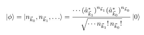
We can then write the full state using the multi mode creation operators:
Now because we know that $\Psi_{x}$ takes $N \to N-1$ particle states, we can simply consider $id_{N-1}$
(note the small abuse of notation. We are not writing the full fock space, rather it is understood that all other alternatives with more or less particles are implied)
$$\bra \psi \rho_{x}\ket \phi = \bra\psi \Psi_{x}^{\dagger}\Psi_{x} \ket \psi = \bra\psi \Psi_{x}^{\dagger}\int dx_{1}dx_{N-1} \ket{\xton{N-1} x} \bra{\xton{N-1}} \Psi_{x} \ket \psi$$
We can pull out the integral (linearity)
$$ = \int dx_{1}dx_{N-1}\bra\psi \Psi_{x}^{\dagger} \ket{\xton{N-1}} \bra{\xton{N-1}} \Psi_{x} \ket \psi$$
We know that $\Psi_{x}^\dagger$ creates a particle at $x$
$$ = N\int dx_{1}dx_{N-1}\bra\psi \ket{\xton{N-1}, x} \bra{\xton{N-1}, x} \ket \psi$$
Now we need to consider all the ways that the states can overlap with the new $x$. We do this by counting the number of times we can have potential overlap. This happens every time, when one of the $x_{i}$ integration variables crosses $x$.
$$ = \sum\limits_{i}^{N}\int dx_{1}dx_{N-1}\bra\psi \ket{\xton{N}} \bra{\xton{N}} \ket \psi \delta(x_{i} - x)$$
We now do something slightly technical. We extend our dirac delta to a distribution acting on operators.
Assuming we already extended it we would like to have
$\delta(\hat x_{i}- x)\ket{\xton{N}} = \delta(x_{i}-x) \ket{\xton{N}}$
I.e. we want it to be compatible with the normal dirac delta.
This will allow us to pull the delta into the integral
$$ = \sum\limits_{i}^{N}\int dx_{1}dx_{N-1}\bra\psi\delta(\hat x_{i} - x) \ket{\xton{N}} \bra{\xton{N}} \ket \psi $$
Why did we do this. Because now $\hat x_{i}$ is no longer an integration variable (it's a distribution).
We can thus take it out of the integral entirely
$$ =\bra\psi \sum\limits_{i}^{N}\delta(\hat x_{i}- x) \underbrace{\int dx_{1}dx_{N-1} \ket{\xton{N}} \bra{\xton{N}}}_{id} \ket \psi $$
We notice the resolution of identity
$$=\bra \psi \sum\limits_{i}^{N} \delta(\hat x_{i}- x) \ket \phi$$
In this form we see directly that we extract for every particle the probability of $\phi$ to be at $x$. And then overlap that with $\psi$
One noteworthy thing is that for $\phi, \psi$ having different numbers of particles, $\delta$ will only stay within the $\phi_N$ block of the matrix.
The overlap will thus always be zero
### Interpretation
If $\phi = \psi$
We see that we count (for every particle) the probability of one of the particles to be at $x$.
That means we calculate the total probability for any particle to be at $x$.
That is exactly the expected density.
# Bose gasses
We want to figure out what happens if we cool down a gas of bosons to near their ground state.
We know that the pauli principle does not apply, so we expect some strange quantum behaviour to occur.
## Pair correlation
To quantify this we introduce the pair correlation function. This function will tell us how "synced up" our particles are.
We first step back and think about what our density operator told us.
$\rho_{x}$ tells us how likely it is for a particle to be at $x$.
Or if we want to be complicated about this. How likely is it that the particle is at $x$ at the same time that it is at $x$. (wooooow)
But there is no reason, why we should not be able to do the same with two particles. For two particles we obviously have two variables $x$ and $y$
The question would now be how likely is it to find one particle at $x$ while the other particle is at $y$.
We first consider an easier model
### Concept question
What is the interpretation of the following operators:
**a)** $\ad \a$
**b)** $\ad_{j}\ad_{i}\a_{i}\a_{j}$
**c)** $\ad_{i}\a_{i}\ad_{j}\a_{j}$
### Concept question
What would be the natural way to build the pair correlation function for the field operators?
It turns out that this is exactly the right notion.
Because we would like this to be a pair density (and probabilities are unitless)
we set $C = \frac{N^{2}}{V^{2}}$
### Fourier modes
There is a nice way to put the mode picture and the field operator picture together. You have done this in the lecture and I'll only quickly outline the process.
- Take some volume $V$
- Find all modes that fit into $V$
- Do the inverse process that we did when deriving the field operator (fourier transform)
- You now know what the density of a mode is
- Link the addition of particles in real space, to the excitation of modes in fourier space
- The creation and destruction of fourier modes are the $\ad_{i}$ and $\a_{i}$
##### Just density
We first write:
$\phi_{j} = \frac{1}{\sqrt{V}}e^{ik_{j}x}$
We can then write the full state using the multi mode creation operators:
 Computing the expectation of a density operator:
$\bra \phi \rho \ket \phi = \bra \phi \Psi^{\dagger}\Psi \ket \phi = \frac{1}{V} \sum\limits_{k_{1},k_{2}} e^{-i(k_{1}-k_{2})x} \bra\phi \ad_{k_{1}} \a_{k_{2}} \ket \phi$
Here we have used the definition of the density operator with respect to the density functions.
Computing the expectation of a density operator:
$\bra \phi \rho \ket \phi = \bra \phi \Psi^{\dagger}\Psi \ket \phi = \frac{1}{V} \sum\limits_{k_{1},k_{2}} e^{-i(k_{1}-k_{2})x} \bra\phi \ad_{k_{1}} \a_{k_{2}} \ket \phi$
Here we have used the definition of the density operator with respect to the density functions.
 Using
$\bra\phi \ad_{k_{1}} \a_{k_{2}} \ket \phi = \delta_{k_{1},k_{2}} n_{k_{1}}$
We can finally write
$\bra \phi \rho \ket \phi = \frac{1}{V}\sum\limits_{k}n_{k} = \frac{N}{V}$
##### Pair correlation
Looking at the form of the density operator
$\bra \phi \rho \ket \phi = \bra \phi \Psi^{\dagger}\Psi \ket \phi = \frac{1}{V} \sum\limits_{k_{1},k_{2}} e^{-i(k_{1}-k_{2})x} \bra\phi \ad_{k_{1}} \a_{k_{2}} \ket \phi$
We notice that there is quite a nice place where we could take our intuitions about the mode correlation and plug them in.
Using a bit of math trickery we thus write
$$\frac{N^{2}}{V^{2}}g(x-y) = \bra \phi \Psi^{\dagger}_{x} \Psi^{\dagger}_{y} \Psi_{y} \Psi_{x} \ket \phi$$
Using
$\bra\phi \ad_{k_{1}} \a_{k_{2}} \ket \phi = \delta_{k_{1},k_{2}} n_{k_{1}}$
We can finally write
$\bra \phi \rho \ket \phi = \frac{1}{V}\sum\limits_{k}n_{k} = \frac{N}{V}$
##### Pair correlation
Looking at the form of the density operator
$\bra \phi \rho \ket \phi = \bra \phi \Psi^{\dagger}\Psi \ket \phi = \frac{1}{V} \sum\limits_{k_{1},k_{2}} e^{-i(k_{1}-k_{2})x} \bra\phi \ad_{k_{1}} \a_{k_{2}} \ket \phi$
We notice that there is quite a nice place where we could take our intuitions about the mode correlation and plug them in.
Using a bit of math trickery we thus write
$$\frac{N^{2}}{V^{2}}g(x-y) = \bra \phi \Psi^{\dagger}_{x} \Psi^{\dagger}_{y} \Psi_{y} \Psi_{x} \ket \phi$$
 Figuring out what the overlap using the creation operators is and after a buch of maths.
The final result is then:
$$\frac{N^{2}}{V^{2}}g(x-y) = \frac{N^{2}}{V^{2}} + \left| \frac{1}{V} \sum\limits_{k}e^{-ik(x-y)} n_{k} \right|^{2} - \frac{1}{V^{2}} \sum\limits_{k}n_{k}(n_{k}+1)$$
## Boson collective states
### Coherent states
Consider the state where all particles are in the same mode
$$\frac{N^{2}}{V^{2}}g(x-y) = \frac{N^{2}}{V^{2}} + \left|\frac{1}{V} \sum\limits_{k} e^{ik(x-y) } N \delta_{k,k_{0}}\right|^{2} - N\frac{N+1}{V^{2}}$$
$$\frac{N^{2}}{V^{2}}g(x-y) = \frac{N^{2}}{V^{2}} + \frac{N^{2}}{V^{2}} - N\frac{N+1}{V^{2}} = \frac{N(N-1)}{V^{2}}$$
We see that the correlation is constant.
That means that there is no correlation between particles.
This might be slightly unintuitive. If they are all in the same state, shouldn't they be **fully** correlated?
The thing is that in the case where all particles are in the same state, the maximum confusion we can have is due to the quantum wave function.
This confusion we cannot reduce without breaking uncertainty.
### Gaussian incoherent states
We consider the state:
$n_{k} = \frac{N}{V} \frac{(2\pi)^{3}}{(b\sqrt{\pi})^{3}}e^\frac{-(k-k_{0})^{2}}{b^{2}}$
We will assume large $V$ so we can replace the sum over an integral
$$\frac{N^{2}}{V^{2}}g(x-y) = \frac{N^{2}}{V^{2}} + \left|\int \frac{d^{3}k}{(2\pi)^{3}} e^{ik(x-y) } \frac{N}{V} \frac{(2\pi)^{3}}{(b\sqrt{\pi})^{3}}e^{\frac{-(k-k_{0})^{2}}{b^{2}}} \right|^{2} - \frac{N^{2}}{V^{2}} \mathcal O(\frac{1}{V})$$
Doing the gaussian integral
we get:
Figuring out what the overlap using the creation operators is and after a buch of maths.
The final result is then:
$$\frac{N^{2}}{V^{2}}g(x-y) = \frac{N^{2}}{V^{2}} + \left| \frac{1}{V} \sum\limits_{k}e^{-ik(x-y)} n_{k} \right|^{2} - \frac{1}{V^{2}} \sum\limits_{k}n_{k}(n_{k}+1)$$
## Boson collective states
### Coherent states
Consider the state where all particles are in the same mode
$$\frac{N^{2}}{V^{2}}g(x-y) = \frac{N^{2}}{V^{2}} + \left|\frac{1}{V} \sum\limits_{k} e^{ik(x-y) } N \delta_{k,k_{0}}\right|^{2} - N\frac{N+1}{V^{2}}$$
$$\frac{N^{2}}{V^{2}}g(x-y) = \frac{N^{2}}{V^{2}} + \frac{N^{2}}{V^{2}} - N\frac{N+1}{V^{2}} = \frac{N(N-1)}{V^{2}}$$
We see that the correlation is constant.
That means that there is no correlation between particles.
This might be slightly unintuitive. If they are all in the same state, shouldn't they be **fully** correlated?
The thing is that in the case where all particles are in the same state, the maximum confusion we can have is due to the quantum wave function.
This confusion we cannot reduce without breaking uncertainty.
### Gaussian incoherent states
We consider the state:
$n_{k} = \frac{N}{V} \frac{(2\pi)^{3}}{(b\sqrt{\pi})^{3}}e^\frac{-(k-k_{0})^{2}}{b^{2}}$
We will assume large $V$ so we can replace the sum over an integral
$$\frac{N^{2}}{V^{2}}g(x-y) = \frac{N^{2}}{V^{2}} + \left|\int \frac{d^{3}k}{(2\pi)^{3}} e^{ik(x-y) } \frac{N}{V} \frac{(2\pi)^{3}}{(b\sqrt{\pi})^{3}}e^{\frac{-(k-k_{0})^{2}}{b^{2}}} \right|^{2} - \frac{N^{2}}{V^{2}} \mathcal O(\frac{1}{V})$$
Doing the gaussian integral
we get:
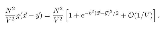 Which is large for $x$ close to $y$ and small far away:
This means that photons (in this state) tend to bunch up close to eachother.
This effect is called Hanbury-Brown-Twiss and paved the way to quantum optics (working with the quantum correlations in light).
The effect can be used to measure the coherence properties of a light source.
This can then for example be used to find the diameter of a star (beyond the resolution limit)
Which is large for $x$ close to $y$ and small far away:
This means that photons (in this state) tend to bunch up close to eachother.
This effect is called Hanbury-Brown-Twiss and paved the way to quantum optics (working with the quantum correlations in light).
The effect can be used to measure the coherence properties of a light source.
This can then for example be used to find the diameter of a star (beyond the resolution limit)