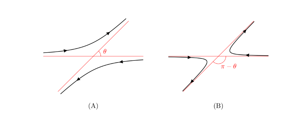
 So the two scattering angles:$\theta$ and $\pi -\theta$ are indistinguishable
We treat the system in the center of momentum frame:
$x_{c}= \frac{x_{1}+x_{2}}{2}$
$x_{r}= x_{1}-x_{2}$
With a new wavefunction $\phi(x_{c},x_{r})$
We assume that this new wavefunction decomposes into a center of momentum and a relative part.
The relative part now is a typical wavefunction we know (and love) from scattering theory.
We can thus write it as the superposition of an incoming planewave and an outgoing (almost) spherical wave.
$$\phi_{r}= \underbrace{e^{i\vec k\vec x}}_{\phi_{in}} + \underbrace{\frac{e^{ik|x|}}{|x|}f(\theta)}_{\phi_{out}}$$
So far we have not considered the symmetry of this wave.
We now need to ask the question whether our $\phi$ needs to be symmetric or antisymmetric. I.e. if the wavefunction is bosonic or fermionic.
So the two scattering angles:$\theta$ and $\pi -\theta$ are indistinguishable
We treat the system in the center of momentum frame:
$x_{c}= \frac{x_{1}+x_{2}}{2}$
$x_{r}= x_{1}-x_{2}$
With a new wavefunction $\phi(x_{c},x_{r})$
We assume that this new wavefunction decomposes into a center of momentum and a relative part.
The relative part now is a typical wavefunction we know (and love) from scattering theory.
We can thus write it as the superposition of an incoming planewave and an outgoing (almost) spherical wave.
$$\phi_{r}= \underbrace{e^{i\vec k\vec x}}_{\phi_{in}} + \underbrace{\frac{e^{ik|x|}}{|x|}f(\theta)}_{\phi_{out}}$$
So far we have not considered the symmetry of this wave.
We now need to ask the question whether our $\phi$ needs to be symmetric or antisymmetric. I.e. if the wavefunction is bosonic or fermionic.
Note that that is a different question than asking if the particle is a boson or a fermion!
We first consider how the relative and centered part of the wavefunction act when permuted.
We find that
- The center stays the same
- The relative coordinate picks up a negative sign
i.e.
$P_{12} \phi(x_{c},x_{r}) = \phi(x_{c},-x_{r})$
That means that the relative part "inherits" the full symmetry / antisymmetry of $\phi$.
More concretely:
If $\phi_{r}$ is an even function, $\phi$ will be symmetric under exchange.
If $\phi_{r}$ is an odd function, $\phi$ will be antisymmetric under exchange.
#### Building the wavefunction
Let's consider building a symmetric relative wavefunction
This means we want to extract the even part of the the wavefunctions.
$\phi_{r} = \frac{1}{C}[\phi_{in}(x) + \phi_{in}(-x)] + \frac{1}{C}[\phi_{out}(x) + \phi_{out}(-x)]$
Sidenote: You can also see this directly by using the symmetrization formula.
($\phi_{sym}= \phi(x) + P_{12}\phi(x)$)
The same is true for antisymmetrization:
$\phi_{r} = \frac{1}{C}[\phi_{in}(x) - \phi_{in}(-x)] + \frac{1}{C}[\phi_{out}(x) - \phi_{out}(-x)]$
Writing this in the explicit form for $\phi_{in}$ and $\phi_{out}$
$\phi_{in}= \frac{1}{C} [e^{ikx} \pm e^{-ikx}]$
$\phi_{out} = \frac{e^{ik|x|}}{|x|} \frac{1}{C} [f(\theta) \pm f(\pi-\theta)]$
In $\phi_{out}$ we now see that all the ingredients are there to mix the two scattering scenarios.
#### Normalization
Because we are dealing with free space waves, which are not normalizable we need to quickly consider what $C$ should be.
Previously we realized that the relevant quantity is not the absolute value, but rather the ratio of input to output. We can thus arbitrarily rescale our wavefunction.
A common convention in to give the input a probability density of $1$.
Doing the math then gives us $C = \sqrt{2}$
#### What symmetrization to choose?
Just as a small recap let's try and think about what symmetrization/antisymmetrization we should choose for certain scenarios.
##### Concept question
Consider the scattering of two electrons with spin up. What symmetry do we choose ($+$ or $-$)
Consider the scattering of two $^{4}He$ atoms in its groundstate. what symmetry do we choose?
#### Differential scattering cross-section
Symmetrizing the scattering cross-section $\dd{\sigma}{\Omega}$
we get:
$$\dd{\sigma}{\Omega}(\theta) = \frac{1}{2}|f(\theta) \pm f(\pi - \theta)|^{2} $$
We see that for $\theta = \frac{\pi}{2}$ and for antisymmetric wavefunctions (-) we get no scattering amplitude.
This is for example the case for fermions in the tripplet state. (symmetric spin, antisymmetric space)
## Second quantisation
For second quantisation we now have a small problem. We initially defined the symmterization over a fixed number of particles.
This allowed us to write the full hilbert space as $S^{n}H$, but now we no longer know how many particles there will be.
What we can now do is we build the tensor algebra (also see linalg II)
 Essentially what we do is we allow any number of particles to be combined.
Mathematically what we do is we create block diagonal matrices of the form:
[[Excalidraw/Wo10_QM_II 2026-04-28 11.17.06.excalidraw.svg]]
Essentially what we do is we allow any number of particles to be combined.
Mathematically what we do is we create block diagonal matrices of the form:
[[Excalidraw/Wo10_QM_II 2026-04-28 11.17.06.excalidraw.svg]]
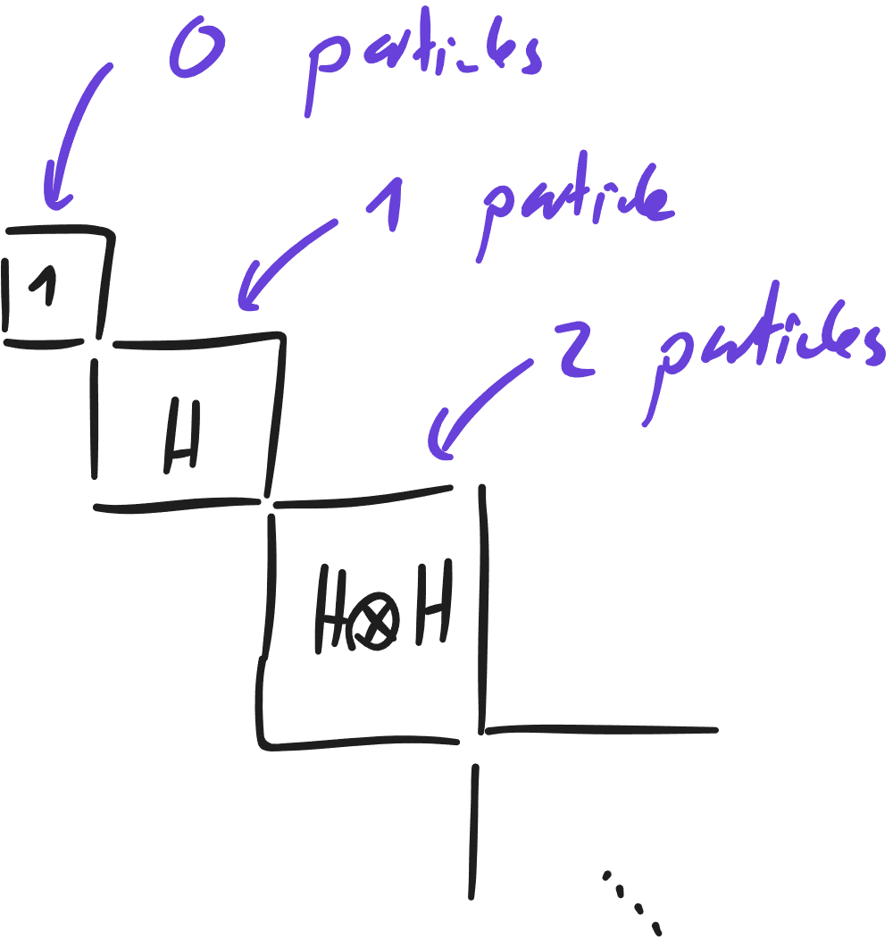 We then treat each subblock as above.
In case we need symmetry we just replace the subblocks with their respective symmetrized block.
The cool thing now is that we can write superpositions (linear combinations) of states with differing numbers of particles.
One thing we need to be careful about is normalization, because the number of particles is not constant.
### Creation / Anihilation
The creation and annihilation operators now jump between the different diagonal blocks:
We then treat each subblock as above.
In case we need symmetry we just replace the subblocks with their respective symmetrized block.
The cool thing now is that we can write superpositions (linear combinations) of states with differing numbers of particles.
One thing we need to be careful about is normalization, because the number of particles is not constant.
### Creation / Anihilation
The creation and annihilation operators now jump between the different diagonal blocks:
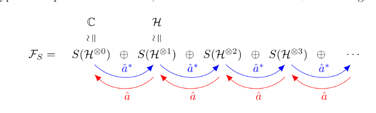 While this seems mathematically overcomplicated it is the minimal structure we need to fully represent many particle systems with variable particle number.
Think back to the harmonic oscillator, which we could represent using the number states $\ket 0 \to \ket N$
Here the creation and anihilation operators are much simpler, and do not nessecitate this "block jumping"
However the harmonic oscillator is also missing the most important feature of the second quantized system:
The particles position.
The point is that in a many body system we will treat states of the type:
$\ket 1 \ket {f_{1}(x)} + \ket 2 \ket {f_{2}(x,y)} + \ldots$
You can now more clearly see the structure, and why we need blocks of differing sizes.
If we have more particles we also need more wavefunctions.
## Spinless Bosons
We want to figure out how to build such states. We lean on a concept we previously know from the HO. The ladder operators.
We would like our ladder operator to create a new particle. However we would also like to be able to choose "what type" of particle we create.
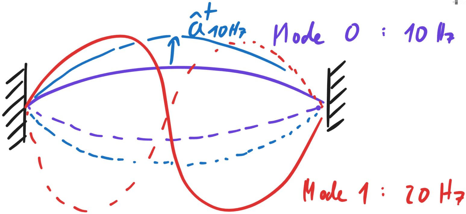
We thus define the mode creation operator $\hat a_{i}^{\dagger}$, which creates a particle in mode $i$.
One picture you can have for this is a single string instrument.
You can have many different higher order modes with differing frequencies. The thing that is quantized is now the amplitude of each mode.
Note that there are "two quantization directions", one is the frequency (first quantisation), the second is the amplitude (second quantisation).
The mode creation operator $\hat a_{10Hz}^{\dagger}$ would thus add one quantum of energy to the mode at $10Hz$.
[[Excalidraw/Wo11_QM_II 2026-05-05 09.43.30.excalidraw.svg]]
While this seems mathematically overcomplicated it is the minimal structure we need to fully represent many particle systems with variable particle number.
Think back to the harmonic oscillator, which we could represent using the number states $\ket 0 \to \ket N$
Here the creation and anihilation operators are much simpler, and do not nessecitate this "block jumping"
However the harmonic oscillator is also missing the most important feature of the second quantized system:
The particles position.
The point is that in a many body system we will treat states of the type:
$\ket 1 \ket {f_{1}(x)} + \ket 2 \ket {f_{2}(x,y)} + \ldots$
You can now more clearly see the structure, and why we need blocks of differing sizes.
If we have more particles we also need more wavefunctions.
## Spinless Bosons
We want to figure out how to build such states. We lean on a concept we previously know from the HO. The ladder operators.
We would like our ladder operator to create a new particle. However we would also like to be able to choose "what type" of particle we create.
We thus define the mode creation operator $\hat a_{i}^{\dagger}$, which creates a particle in mode $i$.
One picture you can have for this is a single string instrument.
You can have many different higher order modes with differing frequencies. The thing that is quantized is now the amplitude of each mode.
Note that there are "two quantization directions", one is the frequency (first quantisation), the second is the amplitude (second quantisation).
The mode creation operator $\hat a_{10Hz}^{\dagger}$ would thus add one quantum of energy to the mode at $10Hz$.
[[Excalidraw/Wo11_QM_II 2026-05-05 09.43.30.excalidraw.svg]]
 We would like to be able to add one particle, no matter how many (or which type) paricles we already have in the system.
I.e.
We want:
$a^{\dagger}_{i}\ket {\phi_{N}} = \sqrt{N+1} \hat S \ket {\phi_{N}} \ket{\psi{i}}$
The prefactor is a normalization constant, and $\hat S$ is there to ensure the proper symmetry.
An easyer way to write the same system is to use the number basis.
We define:
$$\ket{n_{1},\ldots} = \sqrt{\frac{N!}{n_{1}!n_{2}!\cdots}}\hat S \ket\psi_{i} \cdots \ket \psi_{N}$$
Where $n_{i}$ is the number of times the wavefunction $\ket\psi_{i}$ occurs.
In this basis the creation operator is much simpler, and acts as:
$$\hat a^{\dagger}_{i} \ket {n_{1}, \ldots } =\sqrt{n_{i} +1} \ket{n_{1}, \ldots ,n_{i}+1 , \ldots }$$
We can now create states the exact way we are used to:
We would like to be able to add one particle, no matter how many (or which type) paricles we already have in the system.
I.e.
We want:
$a^{\dagger}_{i}\ket {\phi_{N}} = \sqrt{N+1} \hat S \ket {\phi_{N}} \ket{\psi{i}}$
The prefactor is a normalization constant, and $\hat S$ is there to ensure the proper symmetry.
An easyer way to write the same system is to use the number basis.
We define:
$$\ket{n_{1},\ldots} = \sqrt{\frac{N!}{n_{1}!n_{2}!\cdots}}\hat S \ket\psi_{i} \cdots \ket \psi_{N}$$
Where $n_{i}$ is the number of times the wavefunction $\ket\psi_{i}$ occurs.
In this basis the creation operator is much simpler, and acts as:
$$\hat a^{\dagger}_{i} \ket {n_{1}, \ldots } =\sqrt{n_{i} +1} \ket{n_{1}, \ldots ,n_{i}+1 , \ldots }$$
We can now create states the exact way we are used to:
 ### Operators:
We now have some useful operator identies:
$n_{i}= a^{\dagger}_{i}a_{i}$
$N = \sum\limits n_{i}$
$[a_{i}, a_{j}] = 0$
$[a^{\dagger}_{i}, a^{\dagger}_{j}] = 0$
$[a_{i}, a^{\dagger}_{j}] = \delta_{i,j} id$
### Interpretation
At this point we should take a step back and see if the object we constructed represents anything physical.
We note that the structure matches the photon exactly.
This legitimizes thinking about the photon as a bosonic particle!
We found this using a very different path than when we quantized the electromagnetic field.
Here we started with the assumption that we understand single particles and enforced symmetry, whereas in the EM case we started with understanding the field and then found it's particle properties.
## Spin 1/2 Fermions
Similarly to the bosonic case we will again consider a creation operator.
$a^{\dagger}_{i}\ket {\phi_{N}} = \sqrt{N+1} \hat A \ket {\phi_{N}} \ket{\psi{i}}$
However now we need to enforce the antisymmetrization
The number states are then:
$\ket{n_{1}\ldots} = \sqrt{N!} \hat A \ket\phi_{N}\ket{\psi_{i}}$
Note that here the order now matters, because of the antisymmetry!
Again we consider the creation operation on an existing state:
$a^{\dagger}_{i} \ket{n_{1}\ldots n_{i}} = \sqrt{(N+1)!} \hat A \ket{\psi_{i1}}\ket{\psi_{i2}}\ldots \ket{\psi_{iN}}\ket{\psi_{i}}$
Note how the creation operator creates the state at the very right. We now need to permute it into place.
Thus we get
$a^{\dagger}_{i} \ket{n_{1}\ldots n_{i}} = \pm \ket{n_{1},\ldots, n_{i}+1,\ldots}$
With the sign depending on the number of permutations needed.
This gives us an interesting property. If we already have a state $\ket{\psi_{i}}$ in our total wavefunction it is uncear if we need an odd or even number of permutations to "put it into place".
It is actually valid to have both an odd and even permutation. This means: $\ket \Psi = -\ket\Psi = 0$
And enforces the pauli principle!
### Operators
We again get some nice operator properties:
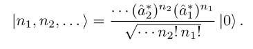
- Creation from vacuum: $\ket{n_{1},n_{2}\ldots} = (a^{\dagger}_{2})^{n_{2}}(a^{\dagger}_{1})^{n_{1}} \ket 0$
- Number operators:
$n_{i}= a^{\dagger}_{i}a_{i}$
$N = \sum\limits n_{i}$
- Commutation relations:
$\{a_{i},a_{j}\} = 0$
$\{a^{\dagger}_{i},a^{\dagger}_{j}\} = 0$
$\{a_{i},a^{\dagger}_{j}\} = \delta_{i,j}id$
Note that we replace the commutator with the anticommutator:
$\{A,B\} = AB + BA$
# Field operators
We figured out how to create particles, however those particles right now are not particularly useful.
The reason for this is that we can currently only create particles in specific modes.
However the interesting quantum mechanics happens exactly when you don't work in eigenmodes.
One thing that would be interesting is to create particles at specified positions
Operators that can do this are called _Field operators_
## Repe: What is a basis
In Qm we always work with an orthonormal basis on some hilbert space.
Orthonormal meaning that $\ket i \perp \ket j$ for $i\neq j$
And $\bra i \ket i = 1$
$\bra i \ket j = \delta_{ij}$
The braket notation is very helpful here, because it implicitly gives us a scalar product, and also a dual basis $\bra 0 \to \bra N$
The property of the dual basis is that it extracts the prefactor of the element dual to it, i.e.
$$l_{0}(\pmatrix{1 \\ 3 \\ 4}) = 1$$
$$l_{1}(\pmatrix{1 \\ 3 \\ 4}) = 3$$
Or much simpler via the dot product:
$$\pmatrix{1 & 0 & 0}\cdot \pmatrix{1 \\ 3 \\ 4} = 1$$
$$\pmatrix{0 & 1 & 0}\cdot \pmatrix{1 \\ 3 \\ 4} = 3$$
If we write a state we can always represent it as a combination of basis vectors (duh)
$\ket f = \sum\limits_{i} c_{i}\ket {i}$
But now we also know how to get the prefactors $c_{i}$ in any basis.
$c_{i}= \bra i \ket f$
We can verify this by calculating explicitly:
$$\bra {i'}\ket f = \sum\limits_{i} \bra {i'} c_{i}\ket {i} = c_{i'}$$
Which is exactly the expected result.
Plugging this back into the original formula for $\ket f$ we get
$\ket f = \sum\limits_{i} \ket i \bra i \ket f$
Thus:
$\sum\limits\ket i \bra i = id$
In matrix form this is not surprising at all:
$\pmatrix{1 \\ 0} \cdot \pmatrix{1 & 0} +\pmatrix{0 \\ 1} \cdot \pmatrix{0 & 1} = \pmatrix{1 & 0 \\ 0 &1}$
### Domain expansion!
We now need to let go of the notion of a finite vector space, because it turns out that hilbert spaces can be uncountable.
We thus transfer our intuitions into the more complicated form.
$\sum\limits \to \int$
All previous identities are still true, however we now index using the continuous variable $y$ instead of the discrete variable $i$.
$\bra g \ket f = \int d^{3}y g(y)^{\star}f(y)$
$\bra x \ket y = \delta_{x-y}$
$\int \ket x \bra x dx = id$
## Localizing a particle
We now want to define an operator that creates a localized position state. ie.
$\Psi^{\dagger}_{x} \ket 0 = \ket x$
We already know how to create modes, if we can mange to express this field operator as a combination of modes we can avoid having to do the full derivation from scratch again.
We consider:
$\bra i \Psi_{x}^{\dagger}\ket 0 = \bra i \ket x = \psi_{i}^{\star}(x)$
(This matrix element corresponds to the h.c. position basis wavefunction of the state $i$)
Consider:
$\sum\limits_{i} \ket i \bra i \Psi_{x}^{\dagger}\ket 0 = \Psi_{x}^{\dagger}\ket 0$
but also
$\sum\limits_{i} \ket i \psi_{i}^{\star}(x) = \Psi_{x}^{\dagger}\ket 0$
Which gives us:
$\sum\limits_{i} \psi_{i}^{\star}(x) a^{\dagger}_{i}\ket 0= \Psi_{x}^{\dagger}\ket 0$
So we can express the field operator as:
$$\Psi_{x}^{\dagger} = \sum\limits_{i}\psi_{i}^{\star}(x) a^{\dagger}_{i}$$
And equivalently for the destruction operator
$$\Psi_{x} = \sum\limits_{i}\psi_{i}(x) a_{i}$$
## Putting it into context
This is not the first time we see field creation operators.
For the vector potential we also found something similar we had:
$$\vec{\hat A}(\vec x) = \frac{1}{\sqrt{L^{3}}} \sum\limits_{k,\lambda} \sqrt{\frac{2\pi\hbar c^{2}}{\omega_{k}}}\left(\hat a_{k,\lambda} \vec e_{k,\lambda} e^{ikx} + h.c. \right)$$
Here however we had a sum of $a$ and $a^{\dagger}$
We did this because $a$ is not hermitian by itself. To get a real observable you need to "balance" it using the h.c.
An other interesting note is that the prefactors in the vector potentials are planewaves $e^{ikx}$. By comparing coefficients we now know that the position space representation of the eigenstates $\ket i$ are also planewaves.
### Operator properties (again)
Now that we have fields, and we understand how bosons and fermions work, we can see that all those notions can be made compatible.
For this we will introduce the double commutator, which allows us to write both bosons and fermions at the same time:
$[A,B]_{\pm} = AB \pm BA$
For different positions we have commutation (locality)
### Operators:
We now have some useful operator identies:
$n_{i}= a^{\dagger}_{i}a_{i}$
$N = \sum\limits n_{i}$
$[a_{i}, a_{j}] = 0$
$[a^{\dagger}_{i}, a^{\dagger}_{j}] = 0$
$[a_{i}, a^{\dagger}_{j}] = \delta_{i,j} id$
### Interpretation
At this point we should take a step back and see if the object we constructed represents anything physical.
We note that the structure matches the photon exactly.
This legitimizes thinking about the photon as a bosonic particle!
We found this using a very different path than when we quantized the electromagnetic field.
Here we started with the assumption that we understand single particles and enforced symmetry, whereas in the EM case we started with understanding the field and then found it's particle properties.
## Spin 1/2 Fermions
Similarly to the bosonic case we will again consider a creation operator.
$a^{\dagger}_{i}\ket {\phi_{N}} = \sqrt{N+1} \hat A \ket {\phi_{N}} \ket{\psi{i}}$
However now we need to enforce the antisymmetrization
The number states are then:
$\ket{n_{1}\ldots} = \sqrt{N!} \hat A \ket\phi_{N}\ket{\psi_{i}}$
Note that here the order now matters, because of the antisymmetry!
Again we consider the creation operation on an existing state:
$a^{\dagger}_{i} \ket{n_{1}\ldots n_{i}} = \sqrt{(N+1)!} \hat A \ket{\psi_{i1}}\ket{\psi_{i2}}\ldots \ket{\psi_{iN}}\ket{\psi_{i}}$
Note how the creation operator creates the state at the very right. We now need to permute it into place.
Thus we get
$a^{\dagger}_{i} \ket{n_{1}\ldots n_{i}} = \pm \ket{n_{1},\ldots, n_{i}+1,\ldots}$
With the sign depending on the number of permutations needed.
This gives us an interesting property. If we already have a state $\ket{\psi_{i}}$ in our total wavefunction it is uncear if we need an odd or even number of permutations to "put it into place".
It is actually valid to have both an odd and even permutation. This means: $\ket \Psi = -\ket\Psi = 0$
And enforces the pauli principle!
### Operators
We again get some nice operator properties:
- Creation from vacuum: $\ket{n_{1},n_{2}\ldots} = (a^{\dagger}_{2})^{n_{2}}(a^{\dagger}_{1})^{n_{1}} \ket 0$
- Number operators:
$n_{i}= a^{\dagger}_{i}a_{i}$
$N = \sum\limits n_{i}$
- Commutation relations:
$\{a_{i},a_{j}\} = 0$
$\{a^{\dagger}_{i},a^{\dagger}_{j}\} = 0$
$\{a_{i},a^{\dagger}_{j}\} = \delta_{i,j}id$
Note that we replace the commutator with the anticommutator:
$\{A,B\} = AB + BA$
# Field operators
We figured out how to create particles, however those particles right now are not particularly useful.
The reason for this is that we can currently only create particles in specific modes.
However the interesting quantum mechanics happens exactly when you don't work in eigenmodes.
One thing that would be interesting is to create particles at specified positions
Operators that can do this are called _Field operators_
## Repe: What is a basis
In Qm we always work with an orthonormal basis on some hilbert space.
Orthonormal meaning that $\ket i \perp \ket j$ for $i\neq j$
And $\bra i \ket i = 1$
$\bra i \ket j = \delta_{ij}$
The braket notation is very helpful here, because it implicitly gives us a scalar product, and also a dual basis $\bra 0 \to \bra N$
The property of the dual basis is that it extracts the prefactor of the element dual to it, i.e.
$$l_{0}(\pmatrix{1 \\ 3 \\ 4}) = 1$$
$$l_{1}(\pmatrix{1 \\ 3 \\ 4}) = 3$$
Or much simpler via the dot product:
$$\pmatrix{1 & 0 & 0}\cdot \pmatrix{1 \\ 3 \\ 4} = 1$$
$$\pmatrix{0 & 1 & 0}\cdot \pmatrix{1 \\ 3 \\ 4} = 3$$
If we write a state we can always represent it as a combination of basis vectors (duh)
$\ket f = \sum\limits_{i} c_{i}\ket {i}$
But now we also know how to get the prefactors $c_{i}$ in any basis.
$c_{i}= \bra i \ket f$
We can verify this by calculating explicitly:
$$\bra {i'}\ket f = \sum\limits_{i} \bra {i'} c_{i}\ket {i} = c_{i'}$$
Which is exactly the expected result.
Plugging this back into the original formula for $\ket f$ we get
$\ket f = \sum\limits_{i} \ket i \bra i \ket f$
Thus:
$\sum\limits\ket i \bra i = id$
In matrix form this is not surprising at all:
$\pmatrix{1 \\ 0} \cdot \pmatrix{1 & 0} +\pmatrix{0 \\ 1} \cdot \pmatrix{0 & 1} = \pmatrix{1 & 0 \\ 0 &1}$
### Domain expansion!
We now need to let go of the notion of a finite vector space, because it turns out that hilbert spaces can be uncountable.
We thus transfer our intuitions into the more complicated form.
$\sum\limits \to \int$
All previous identities are still true, however we now index using the continuous variable $y$ instead of the discrete variable $i$.
$\bra g \ket f = \int d^{3}y g(y)^{\star}f(y)$
$\bra x \ket y = \delta_{x-y}$
$\int \ket x \bra x dx = id$
## Localizing a particle
We now want to define an operator that creates a localized position state. ie.
$\Psi^{\dagger}_{x} \ket 0 = \ket x$
We already know how to create modes, if we can mange to express this field operator as a combination of modes we can avoid having to do the full derivation from scratch again.
We consider:
$\bra i \Psi_{x}^{\dagger}\ket 0 = \bra i \ket x = \psi_{i}^{\star}(x)$
(This matrix element corresponds to the h.c. position basis wavefunction of the state $i$)
Consider:
$\sum\limits_{i} \ket i \bra i \Psi_{x}^{\dagger}\ket 0 = \Psi_{x}^{\dagger}\ket 0$
but also
$\sum\limits_{i} \ket i \psi_{i}^{\star}(x) = \Psi_{x}^{\dagger}\ket 0$
Which gives us:
$\sum\limits_{i} \psi_{i}^{\star}(x) a^{\dagger}_{i}\ket 0= \Psi_{x}^{\dagger}\ket 0$
So we can express the field operator as:
$$\Psi_{x}^{\dagger} = \sum\limits_{i}\psi_{i}^{\star}(x) a^{\dagger}_{i}$$
And equivalently for the destruction operator
$$\Psi_{x} = \sum\limits_{i}\psi_{i}(x) a_{i}$$
## Putting it into context
This is not the first time we see field creation operators.
For the vector potential we also found something similar we had:
$$\vec{\hat A}(\vec x) = \frac{1}{\sqrt{L^{3}}} \sum\limits_{k,\lambda} \sqrt{\frac{2\pi\hbar c^{2}}{\omega_{k}}}\left(\hat a_{k,\lambda} \vec e_{k,\lambda} e^{ikx} + h.c. \right)$$
Here however we had a sum of $a$ and $a^{\dagger}$
We did this because $a$ is not hermitian by itself. To get a real observable you need to "balance" it using the h.c.
An other interesting note is that the prefactors in the vector potentials are planewaves $e^{ikx}$. By comparing coefficients we now know that the position space representation of the eigenstates $\ket i$ are also planewaves.
### Operator properties (again)
Now that we have fields, and we understand how bosons and fermions work, we can see that all those notions can be made compatible.
For this we will introduce the double commutator, which allows us to write both bosons and fermions at the same time:
$[A,B]_{\pm} = AB \pm BA$
For different positions we have commutation (locality)
 Essentially all the properties that you would expect to hold, do hold.
We can now also write position states as being created using the field operators:
$\ket {x_{1} \ldots} = \frac{1}{\sqrt{N!}}\Psi_{x1}^{\dagger}\cdots \ket 0$
# Density operator
This is now the first time Renner introduces the density operator, we have already previously touched upon it in the exercise class.
The general idea is to find the probability to find a particle in some state. To do this we try to destroy the particle and then recreate it. If there was no particle to destroy, we will get zero, and thus cannot recreate the particle
$\rho_{x} = \Psi_{x}^{\dagger}\Psi_{x}$
(note that $\ket 0 \neq 0$ )
This $\rho$ is called the density operator, because it's expecation value gives you the probability density of a particle at $x$.
$\bra \psi \rho_{x}\ket \psi = \bra\psi \Psi_{x}^{\dagger}\Psi(x) \ket \psi$
Essentially all the properties that you would expect to hold, do hold.
We can now also write position states as being created using the field operators:
$\ket {x_{1} \ldots} = \frac{1}{\sqrt{N!}}\Psi_{x1}^{\dagger}\cdots \ket 0$
# Density operator
This is now the first time Renner introduces the density operator, we have already previously touched upon it in the exercise class.
The general idea is to find the probability to find a particle in some state. To do this we try to destroy the particle and then recreate it. If there was no particle to destroy, we will get zero, and thus cannot recreate the particle
$\rho_{x} = \Psi_{x}^{\dagger}\Psi_{x}$
(note that $\ket 0 \neq 0$ )
This $\rho$ is called the density operator, because it's expecation value gives you the probability density of a particle at $x$.
$\bra \psi \rho_{x}\ket \psi = \bra\psi \Psi_{x}^{\dagger}\Psi(x) \ket \psi$