 The only two relevant tableaus are the top and bottom one, which correspond to the totaly symmetric and the signum representation.
### Back to QM
In QM we call particles that are totally symmetric w.r.t. exchange: **Bosons**
Ones that are alternating are called:
**Fermions**
Some interesting properties of these particles directly arise from the underlying mathematics
#### Pauli principle
Remember that $dim(S^{n}V) = \pmatrix{dim(V) + n -1 \\ n}$
and $dim(A^{n}V) = \pmatrix{dim(V) \\ n}$
Note that for symmetric particles the dimension is always $\neq 0$ for any $n >0$ and $dim(V) \neq 0$
This means that I can build totally symmetric combinations of any number of bosonic particles, even if the total space for the bosons is small. (So for example if we only have two states we can put all the bosons in the same state)
But note what happens for fermions for $dim(V) < n$
Suddenly the choose operator is no longer defined!
This means that the maximum number of particles that we can antisymmetrically combine is exactly equal to the number of states.
This means we can have at max one fermion per state!
This is the pauli exclusion principle!
## Why care about fermions vs bosons
It turns out that most of physics in the universe is either directly or indirectly dependent on the difference!
#### The spin statistics theorem
Due to some complicated physics it turns out that in 3D any half integer spin particle is a fermion, whereas any integer spin particle is a boson.
This means that electrons are fermions, and photons have integer spin!
This might seem boring, until you realize that you can also apply this to composite systems
#### Clebsh Gordan decomposition
Remember that any tensor product of spins can be decomposed into a direct sum:
$S_{n} \otimes S_{m} = S_{n+m} \oplus \ldots \oplus S_{n-m}$
Example:
Hydrogen atom:
$S_{\frac{1}{2}}^{e-} \otimes S_{\frac{1}{2}}^{p+} = S_{1} \oplus S_{0}$
This means that the hydrogen atom is a boson!
Compare this with deuterium (which contains an additional neutron with spin $\frac{1}{2}$, which is a fermion)
#### Bose einstein condensates
We found that bosons are allowed to occupy the same state. This means that if we cool hydrogen enough such that it is in its ground state, all the hydrogen will be in the same state!
This phenomenon is called bose einstein condensation and is still an active topic of research.
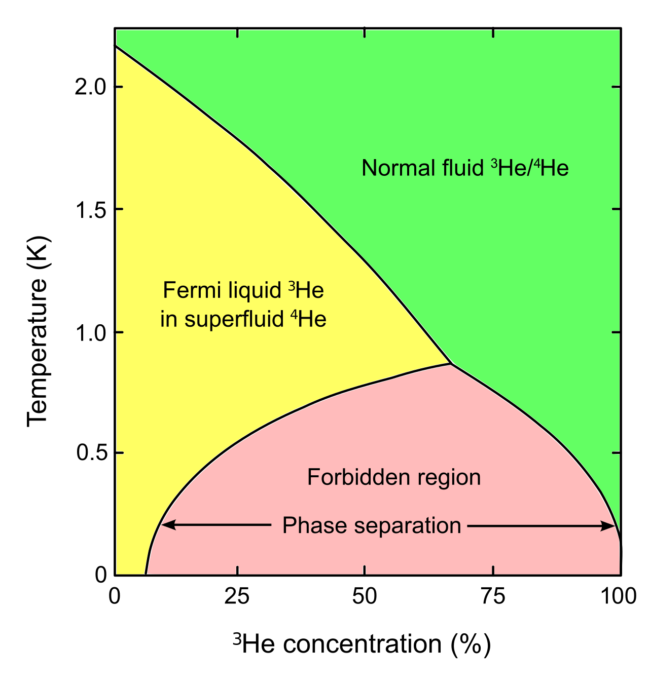
#### Dilution fridges
Ever wondered how you can build a quantum computer?
The only two relevant tableaus are the top and bottom one, which correspond to the totaly symmetric and the signum representation.
### Back to QM
In QM we call particles that are totally symmetric w.r.t. exchange: **Bosons**
Ones that are alternating are called:
**Fermions**
Some interesting properties of these particles directly arise from the underlying mathematics
#### Pauli principle
Remember that $dim(S^{n}V) = \pmatrix{dim(V) + n -1 \\ n}$
and $dim(A^{n}V) = \pmatrix{dim(V) \\ n}$
Note that for symmetric particles the dimension is always $\neq 0$ for any $n >0$ and $dim(V) \neq 0$
This means that I can build totally symmetric combinations of any number of bosonic particles, even if the total space for the bosons is small. (So for example if we only have two states we can put all the bosons in the same state)
But note what happens for fermions for $dim(V) < n$
Suddenly the choose operator is no longer defined!
This means that the maximum number of particles that we can antisymmetrically combine is exactly equal to the number of states.
This means we can have at max one fermion per state!
This is the pauli exclusion principle!
## Why care about fermions vs bosons
It turns out that most of physics in the universe is either directly or indirectly dependent on the difference!
#### The spin statistics theorem
Due to some complicated physics it turns out that in 3D any half integer spin particle is a fermion, whereas any integer spin particle is a boson.
This means that electrons are fermions, and photons have integer spin!
This might seem boring, until you realize that you can also apply this to composite systems
#### Clebsh Gordan decomposition
Remember that any tensor product of spins can be decomposed into a direct sum:
$S_{n} \otimes S_{m} = S_{n+m} \oplus \ldots \oplus S_{n-m}$
Example:
Hydrogen atom:
$S_{\frac{1}{2}}^{e-} \otimes S_{\frac{1}{2}}^{p+} = S_{1} \oplus S_{0}$
This means that the hydrogen atom is a boson!
Compare this with deuterium (which contains an additional neutron with spin $\frac{1}{2}$, which is a fermion)
#### Bose einstein condensates
We found that bosons are allowed to occupy the same state. This means that if we cool hydrogen enough such that it is in its ground state, all the hydrogen will be in the same state!
This phenomenon is called bose einstein condensation and is still an active topic of research.
#### Dilution fridges
Ever wondered how you can build a quantum computer?
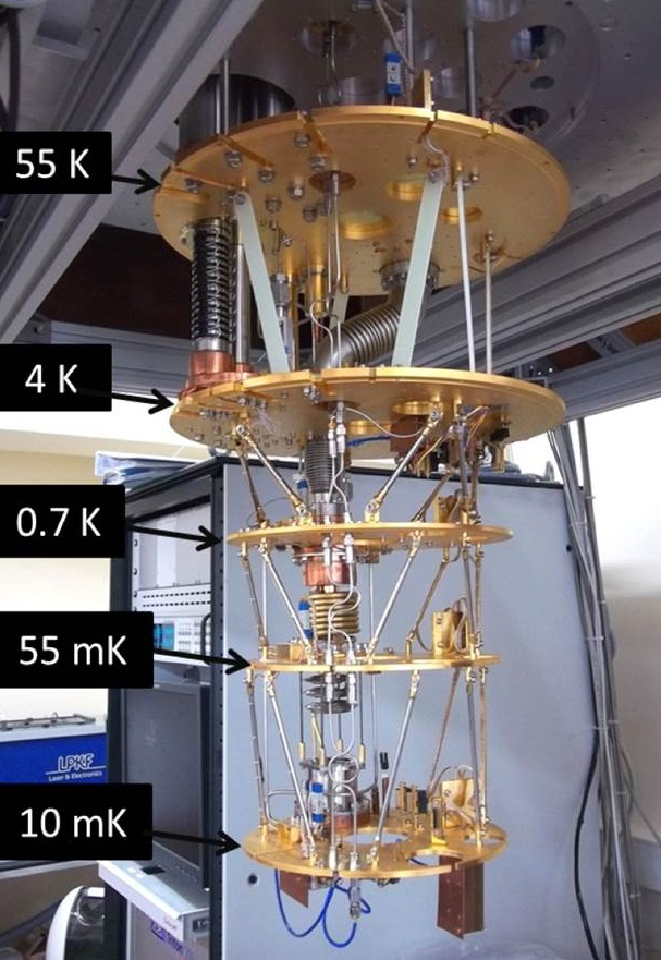 To reach the cold temperatures needed you need to be very clever about extracting heat from the system.
One way this is done in the last stage is a so-called dilution fridge. It works by exploiting the difference in condensation behaviour of $He_{4}$ (a boson) and $He_{3}$ (a fermion)
To reach the cold temperatures needed you need to be very clever about extracting heat from the system.
One way this is done in the last stage is a so-called dilution fridge. It works by exploiting the difference in condensation behaviour of $He_{4}$ (a boson) and $He_{3}$ (a fermion)
 #### Chemistry
Chemistry for example relies on the fact that we have at max 2 electrons per orbital. Without that all electrons would condense into the $1s$ orbital, refusing to interact with other atoms, breaking all of chemistry (and matter as a whole).
#### Technology
Semiconductors rely on the concept of a fermi sea, that is the energy level where electrons "pile up towards". Because not all electrons can be in the ground state we have this bunching up effect.
A semiconductor exploits this by putting a forbidden region between the fermi sea and the next higher energy levels.
Electrons can only start moving if they are given the energy to jump the gap.
This is the basis for photovoltaics, and transistors!
and so much more!
## Symmetrization / Antisymmetrization
Let's say we want to take a general state, which does not yet have the correct symmetry and symmetrize/ antisymmetrize it.
This would be useful in case we know some parts of a state, and also the correct symmetry. In this case we could reconstruct how the rest of the state needs to look like.
We can use the projection formula from representation theory to project onto a specific irrep.
$\hat S \ket \psi = \frac{1}{N!}\sum\limits_{\pi\in S_{N}}\hat P_{\pi}\ket\psi$
$\hat A \ket \psi = \frac{1}{N!}\sum\limits_{\pi\in S_{N}}sgn(\pi)\hat P_{\pi}\ket\psi$
(note how $sgn$ takes the role of the character here)
### Example spin triplets:
Consider a system made from two electrons:
$\psi = \ket{\phi_{\uparrow\uparrow}}\ket{\uparrow\uparrow} + \ket{\phi_{\downarrow\uparrow}} \ket{\downarrow\uparrow} + \ket{\phi_{\uparrow\downarrow}}\ket{\uparrow\downarrow} + \ket{\phi_{\downarrow\downarrow}}\ket{\downarrow\downarrow}$
They each have a spatial as well as a spin component.
We can find that there is one spin 1 subspace and one spin 0 subspace (we could have seen that from clebsh gordan as well)
#### Chemistry
Chemistry for example relies on the fact that we have at max 2 electrons per orbital. Without that all electrons would condense into the $1s$ orbital, refusing to interact with other atoms, breaking all of chemistry (and matter as a whole).
#### Technology
Semiconductors rely on the concept of a fermi sea, that is the energy level where electrons "pile up towards". Because not all electrons can be in the ground state we have this bunching up effect.
A semiconductor exploits this by putting a forbidden region between the fermi sea and the next higher energy levels.
Electrons can only start moving if they are given the energy to jump the gap.
This is the basis for photovoltaics, and transistors!
and so much more!
## Symmetrization / Antisymmetrization
Let's say we want to take a general state, which does not yet have the correct symmetry and symmetrize/ antisymmetrize it.
This would be useful in case we know some parts of a state, and also the correct symmetry. In this case we could reconstruct how the rest of the state needs to look like.
We can use the projection formula from representation theory to project onto a specific irrep.
$\hat S \ket \psi = \frac{1}{N!}\sum\limits_{\pi\in S_{N}}\hat P_{\pi}\ket\psi$
$\hat A \ket \psi = \frac{1}{N!}\sum\limits_{\pi\in S_{N}}sgn(\pi)\hat P_{\pi}\ket\psi$
(note how $sgn$ takes the role of the character here)
### Example spin triplets:
Consider a system made from two electrons:
$\psi = \ket{\phi_{\uparrow\uparrow}}\ket{\uparrow\uparrow} + \ket{\phi_{\downarrow\uparrow}} \ket{\downarrow\uparrow} + \ket{\phi_{\uparrow\downarrow}}\ket{\uparrow\downarrow} + \ket{\phi_{\downarrow\downarrow}}\ket{\downarrow\downarrow}$
They each have a spatial as well as a spin component.
We can find that there is one spin 1 subspace and one spin 0 subspace (we could have seen that from clebsh gordan as well)
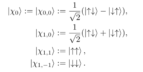 We know that the two electrons are fermions. Thus exchanging them needs to give us a minus.
We also see that the state $\ket \chi_{00}$ is antisymmetric, whereas the others are symmetric under permutation.
To satisfy the symmetry as a _total_ object, the spatial wavefunctions need to compensate for the symmetries of the spin.
From this we find that:
- Singlet states have _symmetric spatial wavefunctions_
- Triplet states have _antisymmetric spatial wavefunctions_
Note this might be slightly confusing, because we have four objects with distinct symmetries:
- The electrons between themselves -> Fermions antisymmetric
- The electron spin -> Follows the symmetry of clebsh gordan (not single symmetry)
- The electron wavefunction -> Adapts to the spin state symmetry to produce the total symmetry
- Two electrons as a pair -> Boson symmetric
## Many particle systems
When we want to describe a system of many particles we can tensor product the operators on the states to get a total system operator.
We often write the total hamiltonian as:
$H = \sum\limits_{j} \tilde H_{j}$
Where we mean that $H_{j}$ only acts on the $jth$ particle.
This is technically abuse of notation, because what we mean is:
$H \in \tilde H ^{\otimes N}$. This would mean that a sum of small operators magically gives us a large operator.
What we actually mean is:
$H = \sum\limits_{j} id_{1} \otimes \ldots \otimes \tilde H{j} \otimes \ldots \otimes id_{N}$
We embed the local operator into the total system energy by saying it acts as $\tilde H_{j}$ on the $j$ system, while acting as the identity on all others.
### Solving the system
In case there are no interactions between the subsystems (which is true by construction) we can solve for the wavefunctions of each particle individually. (We basically diagonalize each Hamiltonian separately, and then combine the unitaries)
The resulting states are thus products of the single particle eigenfunctions.
### Symmetrization
Depending on the statistics of the particles we now need to enforce symmtery.
#### Bosons:
For bosons this is fairly simple, we just product all permutations and normalize.
#### Fermions:
We know that the two electrons are fermions. Thus exchanging them needs to give us a minus.
We also see that the state $\ket \chi_{00}$ is antisymmetric, whereas the others are symmetric under permutation.
To satisfy the symmetry as a _total_ object, the spatial wavefunctions need to compensate for the symmetries of the spin.
From this we find that:
- Singlet states have _symmetric spatial wavefunctions_
- Triplet states have _antisymmetric spatial wavefunctions_
Note this might be slightly confusing, because we have four objects with distinct symmetries:
- The electrons between themselves -> Fermions antisymmetric
- The electron spin -> Follows the symmetry of clebsh gordan (not single symmetry)
- The electron wavefunction -> Adapts to the spin state symmetry to produce the total symmetry
- Two electrons as a pair -> Boson symmetric
## Many particle systems
When we want to describe a system of many particles we can tensor product the operators on the states to get a total system operator.
We often write the total hamiltonian as:
$H = \sum\limits_{j} \tilde H_{j}$
Where we mean that $H_{j}$ only acts on the $jth$ particle.
This is technically abuse of notation, because what we mean is:
$H \in \tilde H ^{\otimes N}$. This would mean that a sum of small operators magically gives us a large operator.
What we actually mean is:
$H = \sum\limits_{j} id_{1} \otimes \ldots \otimes \tilde H{j} \otimes \ldots \otimes id_{N}$
We embed the local operator into the total system energy by saying it acts as $\tilde H_{j}$ on the $j$ system, while acting as the identity on all others.
### Solving the system
In case there are no interactions between the subsystems (which is true by construction) we can solve for the wavefunctions of each particle individually. (We basically diagonalize each Hamiltonian separately, and then combine the unitaries)
The resulting states are thus products of the single particle eigenfunctions.
### Symmetrization
Depending on the statistics of the particles we now need to enforce symmtery.
#### Bosons:
For bosons this is fairly simple, we just product all permutations and normalize.
#### Fermions:
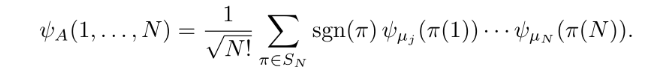 We note that we want all totally asymmetrical combination of $N$ elements. If you remember linalg I we had a similar dream when we constructed the determinant.
$det(A) = \sum\limits_{\sigma\in S_{n}} (sgn(\sigma) \prod_{i} a_{i\sigma_{i}})$
We can thus use the slatter determinand to construct the total antisymmetrization:
We note that we want all totally asymmetrical combination of $N$ elements. If you remember linalg I we had a similar dream when we constructed the determinant.
$det(A) = \sum\limits_{\sigma\in S_{n}} (sgn(\sigma) \prod_{i} a_{i\sigma_{i}})$
We can thus use the slatter determinand to construct the total antisymmetrization:
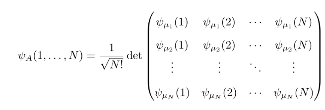 This again shows us the Pauli principle (because the determinant of a matrix with linearly dependent rows (so non-full rank) is always zero)
### The groundstate
This again shows us the Pauli principle (because the determinant of a matrix with linearly dependent rows (so non-full rank) is always zero)
### The groundstate
 ## Scattering
Due to indistinguishably it is now no longer possible to separate the two scenarios below:
## Scattering
Due to indistinguishably it is now no longer possible to separate the two scenarios below:
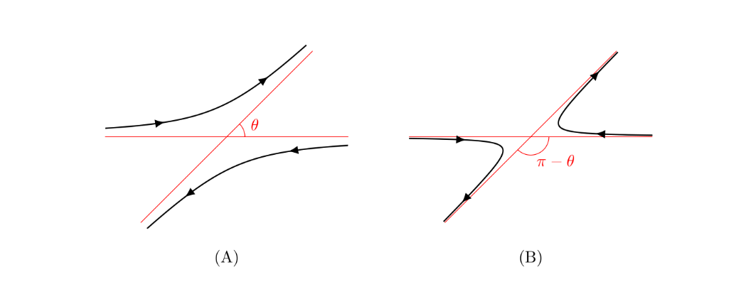 We thus have to symmetrize the scattering amplitudes.
We then get:
For Bosons:
$\phi_{out}(x) = \frac{e^{ikx}}{x} \frac{1}{C}[f(\theta) + f(\theta)]$
And for Fermions:
$\phi_{out}(x) = \frac{e^{ikx}}{x} \frac{1}{C}[f(\theta) - f(\theta)]$
#### Differential scattering cross-section
Symmetrizing the scattering cross-section $\dd{\sigma}{\Omega}$
we get:
$$\dd{\sigma}{\Omega}(\theta) = \frac{1}{2}|f(\theta) \pm f(\pi - \theta)|^{2} $$
We see that for $\theta = \frac{\pi}{2}$ and for fermions (-) we get no scattering amplitude when $f$ is antisymmetric.
This is for example the case for fermions in the tripplet state.
Important sidenote:
- Scattering only interacts with the spatial wavefunction. So to apply the symmetry we not only need to know if we are dealing with a boson or a fermion, but also what the symmetry of the wavefunction is. (because $f$ is the total wavefunction which always consists of two particles)
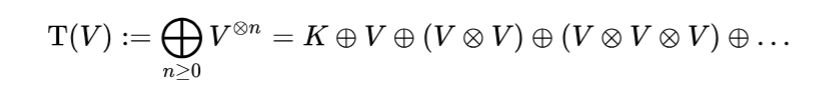
## Second quantisation
For second quantisation we now have a small problem. We initially defined the symmterization over a fixed number of particles.
This allowed us to write the full hilbert space as $S^{n}H$, but now we no longer know how many particles there will be.
What we can now do is we build the tensor algebra (also see linalg II)
We thus have to symmetrize the scattering amplitudes.
We then get:
For Bosons:
$\phi_{out}(x) = \frac{e^{ikx}}{x} \frac{1}{C}[f(\theta) + f(\theta)]$
And for Fermions:
$\phi_{out}(x) = \frac{e^{ikx}}{x} \frac{1}{C}[f(\theta) - f(\theta)]$
#### Differential scattering cross-section
Symmetrizing the scattering cross-section $\dd{\sigma}{\Omega}$
we get:
$$\dd{\sigma}{\Omega}(\theta) = \frac{1}{2}|f(\theta) \pm f(\pi - \theta)|^{2} $$
We see that for $\theta = \frac{\pi}{2}$ and for fermions (-) we get no scattering amplitude when $f$ is antisymmetric.
This is for example the case for fermions in the tripplet state.
Important sidenote:
- Scattering only interacts with the spatial wavefunction. So to apply the symmetry we not only need to know if we are dealing with a boson or a fermion, but also what the symmetry of the wavefunction is. (because $f$ is the total wavefunction which always consists of two particles)
## Second quantisation
For second quantisation we now have a small problem. We initially defined the symmterization over a fixed number of particles.
This allowed us to write the full hilbert space as $S^{n}H$, but now we no longer know how many particles there will be.
What we can now do is we build the tensor algebra (also see linalg II)
 Essentially what we do is we allow any number of particles to be combined.
Mathematically what we do is we create block diagonal matrices of the form:
Essentially what we do is we allow any number of particles to be combined.
Mathematically what we do is we create block diagonal matrices of the form:
 We then treat each subblock as above.
In case we need symmetry we just replace the subblocks with their respective symmetrized block.
The cool thing now is that we can write superpositions (linear combinations) of states with differing numbers of particles.
One thing we need to be careful about is normalization, because the number of particles is not constant.
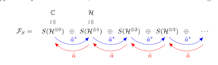
### Creation / Anihilation
The creation and annihilation operators now jump between the different diagonal blocks:
We then treat each subblock as above.
In case we need symmetry we just replace the subblocks with their respective symmetrized block.
The cool thing now is that we can write superpositions (linear combinations) of states with differing numbers of particles.
One thing we need to be careful about is normalization, because the number of particles is not constant.
### Creation / Anihilation
The creation and annihilation operators now jump between the different diagonal blocks: