$\newcommand{\dede}[2]{\frac{\partial #1}{\partial #2} }
\newcommand{\dd}[2]{\frac{d #1}{d #2}}
\newcommand{\divby}[1]{\frac{1}{#1} }
\newcommand{\typing}[3][\Gamma]{#1 \vdash #2 : #3}
\newcommand{\xyz}[0]{(x,y,z)}
\newcommand{\xyzt}[0]{(x,y,z,t)}
\newcommand{\hams}[0]{-\frac{\hbar^2}{2m}(\dede{^2}{x^2} + \dede{^2}{y^2} + \dede{^2}{z^2}) + V\xyz}
\newcommand{\hamt}[0]{-\frac{\hbar^2}{2m}(\dede{^2}{x^2} + \dede{^2}{y^2} + \dede{^2}{z^2}) + V\xyzt}
\newcommand{\ham}[0]{-\frac{\hbar^2}{2m}(\dede{^2}{x^2}) + V(x)}
\newcommand{\konko}[2]{^{#1}\space_{#2}}
\newcommand{\kokon}[2]{_{#1}\space^{#2}} $
# Content
$\newcommand{\L}{\mathcal L}$
### Repe Hamiltonian mechanics
Last week I mentioned that an intuitive way to check compatibility was to do the commutation test.
I need to correct myself on that. The commutation test is sadly not enough.
The actual statement is the following:
$$\{A, B\} = \dede{A}{q}\dede{B}{p} - \dede{A}{p}\dede{B}{q}$$
Which we can write as a product of two vectors:
$$\{A,B\} = \begin{pmatrix} -\dede{A}{p} \\ \dede{A}{q}\end{pmatrix} \cdot \begin{pmatrix}\dede{B}{q} \\ \dede{B}{p}\end{pmatrix} = X_{A}^{T} \nabla B = X_{A}^{T}\begin{pmatrix} 0 & -1 \\ 1 & 0 \end{pmatrix} X_{B}$$
We see that the actual statement for commutation is that the rotated fields are orthogonal. Or alternatively that the original fields are parallel.
> Sketch
#### Why commutation works?
The actual reason why we can have the commutation relations in canonical quantisation is because we _impose_ the quantisation. We then find from that quantisation that there has to be a phase involved when changing between $xp$ and $px$. See later in the lesson
#### Repe Back to matter
At the very end of last week I also mentioned that the reason for the different behaviour of matter waves and light waves was the scaling of the hamiltonian with the energy.
##### The path integral
We saw that the probability of propagation from $q_{i}\to q_{f}$ in $\Delta t$ is given by
$$K(t_{f}-t_{i}, q_{f}, q_{i}) = \int_{q_{i},t_{i}\to q_{f}t_{f}} D\gamma e^{\frac{i}{\hbar}S[\gamma]}$$.
Which has large contributions of a path when $S[\gamma]$ along the path interferes constructively with many other paths.
Now considering that $S[\gamma] = \int_{\gamma} \L ds = \int_{\gamma} (T-V) ds$
For freely propagating particles/ light we have $V=0$
We saw that one way to interpret this term $e^{\frac{i}{\hbar}S[\gamma]}$ is a phase picked up along the path. We want to find how this phase depends on the path.
We had
We see this difference when considering the energy of a photon:
$E = h\nu = \frac{hc}{\lambda} = c p_{\nu}$
Whereas a massive particle will have
$E = \frac{1}{2m}p^{2} =\frac{1}{2m} \frac{h^{2}}{\lambda^{2}}$
We first consider the case for light:
$$\exp\left(\frac{i}{\hbar} \int_{\gamma} \frac{hc}{\lambda}d \gamma\right)= \exp\left(\int_{\gamma}\frac{2\pi i}{\lambda} d\gamma\right) = \exp\left(2\pi i \int_{\gamma} \frac{1}{\dd{x}{\phi}} \dd{\gamma}{x} dx \right)$$
$$\exp\left( 2\pi i \int_{\gamma}\dd{\phi}{x} \dd{\gamma}{x}dx \right)= \exp\left(2\pi i \int_{\gamma} \dd{\gamma}{x}d\phi\right)$$
We note that the total phase now only depends on the length of the path.
Now we consider matter:
$$\exp\left(\frac{i}{\hbar} \int_{\gamma} \frac{h^{2}}{2m \lambda^{2}}d \gamma\right) = \exp \left(2\pi i \int_{\gamma} \frac{h}{2m \dd{x}{\phi}^{2}} \right) = \ldots$$
$$\propto \exp\left(2\pi i \int_{\gamma}\dd{\gamma}{x} \dd{\phi}{x} d\phi\right)$$
Which retains a dependence on the parametrisation of $\phi$.
Meaning the phase we can pick up depends on how fast we move along the path.
Fazit:
- For light the phase picked up along a path only depends on distance, not on the "speed" along which we integrate
- For matter the phase also depends on our parametrisation of the path.
Thus. For light all speed is the same, for matter we have differing speeds.
## Commutators
In class you derived the commutation relation of $x$ and $p$ by formalizing the intuition that you already have about commutators.
Specifically you used the two point correlation function
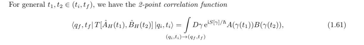 To find what happens if you change the measurement order.
It is useful to note that when we write $[x,p]$ we need to consider that this is an observable. Because we do not know the form of $[x,p]$ yet, we need to assume that this is something we can measure, and more importantly, that we measure at some point in time:
$[x,p](t)$
Now this might be a bit confusing, because using this intuition we would expect:
$[x(t),p(t)]= x(t)p(t)- p(t)x(t) = x(t)p(t)-x(t)p(t)=0$
Because we measure exactly _at the same time_. It should not matter what order we write it in.
The point is that we are not allowed to do this re-ordering without justification.
For this we need a formula that connects the "operational order" with the "temporal order".
This is why we wrote formula (1.61) using the time ordering operator. We only understand qm correctly when the "operational order" is the same as the "temporal order".
I.e. When the oder i measure my things in, is also the order (in time) i do the measurements.
### The derivation
The reason thus why we are doing this strange $\varepsilon$ limiting procedure ist make the two notions of order into the same thing.
## The classical limit
When developing a new theory of physics we always want to remain compatible with the old physics. We thus expect the path integral formalism to decay into classical lagrangian physics when we "remove the quantumnes".
For this we can first wonder which part of our formalism is actually truly quantum.
Historically quantum mechanics was found when Planck used some ad-hoc trick to solve the UV catastrophe. He introduced an energy quantum, which scaled with $\hbar$.
In the limit of $\hbar \to 0$ we would thus expect to get back the classical uv catastrophe (which we get).
So this is a good limit to take.
However we need to keep in mind that this is _one aspect_ of quantumness. It is still an ongoing debate about what is the correct way to do a classical limit.
### The $\hbar$ limit
When working with the path integral we always considered the superposition of infinitely many paths. The phase on these paths was complex (so not an observable).
When we thus ask what path did the particle take, we cannot just say we take the expectation value of $\exp(\frac{i}{\hbar}S[\gamma])$. Observables are real, thus we can never fully trace a quantum path.
This means that if we want to find which quantum path a particle takes, we need to consider the full path at once. (Because this gives us a transition probability, which is real).
In some sense this is the same problem we face when doing a double slit experiment. We would like to know which slit the particle went throuhg, but by measuring at the slit, we enforce real boundry conditions at the slit, thus disturbing the outcome.
#### Path measurements
To avoid setting unnecessary boundry conditions we measure the full path at once. We do this by filling the space with "forbidden zones". If the path goes through a forbidden zone, we consider it "failed."
We can now carve out allowed paths, for which we can then calculate the probability of success.
The meaning of this is then simple. The probability of successfully traveling the path is proportional to the probability of having taken the path.
To find what happens if you change the measurement order.
It is useful to note that when we write $[x,p]$ we need to consider that this is an observable. Because we do not know the form of $[x,p]$ yet, we need to assume that this is something we can measure, and more importantly, that we measure at some point in time:
$[x,p](t)$
Now this might be a bit confusing, because using this intuition we would expect:
$[x(t),p(t)]= x(t)p(t)- p(t)x(t) = x(t)p(t)-x(t)p(t)=0$
Because we measure exactly _at the same time_. It should not matter what order we write it in.
The point is that we are not allowed to do this re-ordering without justification.
For this we need a formula that connects the "operational order" with the "temporal order".
This is why we wrote formula (1.61) using the time ordering operator. We only understand qm correctly when the "operational order" is the same as the "temporal order".
I.e. When the oder i measure my things in, is also the order (in time) i do the measurements.
### The derivation
The reason thus why we are doing this strange $\varepsilon$ limiting procedure ist make the two notions of order into the same thing.
## The classical limit
When developing a new theory of physics we always want to remain compatible with the old physics. We thus expect the path integral formalism to decay into classical lagrangian physics when we "remove the quantumnes".
For this we can first wonder which part of our formalism is actually truly quantum.
Historically quantum mechanics was found when Planck used some ad-hoc trick to solve the UV catastrophe. He introduced an energy quantum, which scaled with $\hbar$.
In the limit of $\hbar \to 0$ we would thus expect to get back the classical uv catastrophe (which we get).
So this is a good limit to take.
However we need to keep in mind that this is _one aspect_ of quantumness. It is still an ongoing debate about what is the correct way to do a classical limit.
### The $\hbar$ limit
When working with the path integral we always considered the superposition of infinitely many paths. The phase on these paths was complex (so not an observable).
When we thus ask what path did the particle take, we cannot just say we take the expectation value of $\exp(\frac{i}{\hbar}S[\gamma])$. Observables are real, thus we can never fully trace a quantum path.
This means that if we want to find which quantum path a particle takes, we need to consider the full path at once. (Because this gives us a transition probability, which is real).
In some sense this is the same problem we face when doing a double slit experiment. We would like to know which slit the particle went throuhg, but by measuring at the slit, we enforce real boundry conditions at the slit, thus disturbing the outcome.
#### Path measurements
To avoid setting unnecessary boundry conditions we measure the full path at once. We do this by filling the space with "forbidden zones". If the path goes through a forbidden zone, we consider it "failed."
We can now carve out allowed paths, for which we can then calculate the probability of success.
The meaning of this is then simple. The probability of successfully traveling the path is proportional to the probability of having taken the path.
 Let's re-examine the form of the path integral:
$$K(t_{f}-t_{i}, q_{f}, q_{i}) = \int_{q_{i},t_{i}\to q_{f}t_{f}} D\gamma e^{\frac{i}{\hbar}S[\gamma]}$$
We see that as $\hbar \to 0$ the number of oscillations per $dS$ diverges. The classical limit is thus the limit where $S$ is really large.
> sketch
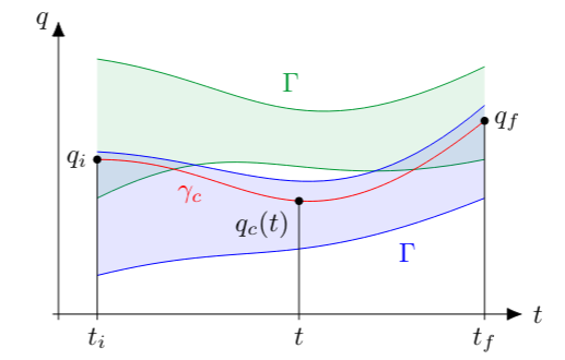
#### The classical path
We can now calculate the path we would expect to see from classical physics.
We consider our limit compatible only when the probability to stay in a tube around the classical path goes to $1$ as $\hbar \to 0$
## Thermodynamics
### Pure vs Mixed states.
In QM we can prepare experiments, and we always get a probability distribution as an outcome.
However the source of the uncertainty is not always the same:
#### Probabilistic classical physics
Consider an experiment where I roll a dice and then do some classical experiment.
I will get a stochastic output from this experiment, however no "quantumnes" was involved.
The fact that we had randomness in our experiment did not prove that classical physics is non-deterministic. The only thing we learned is that we cannot control the system well enough.
#### Intrinsic probability
Contrast this with a position measurement of a momentum eigenstate.
Let's say we can reliably create a momentum eigenstate.
When we measure the position, we still get "random" results.
This is however not due to our inability to prepare a good system, but because of the inherent randomness of quantum mechanics.
#### Combining the two
What if we now have a system with quantum randomness and experimental ("classical" ) randomness.
We can no longer write the two outcomes in a state vector (because that type of randomness is always fully quantum).
We need a new object.
#### The density matrix
In the density matrix we can write both classical as well as quantum uncertainty.
$\rho = \sum\limits_{ij} p_{ij} \ket i \bra j$
It in some sense measures the probability to go from state $j$ to state
## Feedback
https://forms.gle/agfZFxXRTvCUgJiN6
Let's re-examine the form of the path integral:
$$K(t_{f}-t_{i}, q_{f}, q_{i}) = \int_{q_{i},t_{i}\to q_{f}t_{f}} D\gamma e^{\frac{i}{\hbar}S[\gamma]}$$
We see that as $\hbar \to 0$ the number of oscillations per $dS$ diverges. The classical limit is thus the limit where $S$ is really large.
> sketch
#### The classical path
We can now calculate the path we would expect to see from classical physics.
We consider our limit compatible only when the probability to stay in a tube around the classical path goes to $1$ as $\hbar \to 0$
## Thermodynamics
### Pure vs Mixed states.
In QM we can prepare experiments, and we always get a probability distribution as an outcome.
However the source of the uncertainty is not always the same:
#### Probabilistic classical physics
Consider an experiment where I roll a dice and then do some classical experiment.
I will get a stochastic output from this experiment, however no "quantumnes" was involved.
The fact that we had randomness in our experiment did not prove that classical physics is non-deterministic. The only thing we learned is that we cannot control the system well enough.
#### Intrinsic probability
Contrast this with a position measurement of a momentum eigenstate.
Let's say we can reliably create a momentum eigenstate.
When we measure the position, we still get "random" results.
This is however not due to our inability to prepare a good system, but because of the inherent randomness of quantum mechanics.
#### Combining the two
What if we now have a system with quantum randomness and experimental ("classical" ) randomness.
We can no longer write the two outcomes in a state vector (because that type of randomness is always fully quantum).
We need a new object.
#### The density matrix
In the density matrix we can write both classical as well as quantum uncertainty.
$\rho = \sum\limits_{ij} p_{ij} \ket i \bra j$
It in some sense measures the probability to go from state $j$ to state
## Feedback
https://forms.gle/agfZFxXRTvCUgJiN6